How to tune ISP using the STM32 ISP IQTune

1. Article purpose

Unlike a camera module that embeds the lens, the image sensor, and the image signal processor (ISP), the RAW sensor module only embeds the lens and the image sensor.

Information

The image signal processor (ISP) processes the raw data from the sensor to produce a viewable image. It handles tasks such as white balance and color correction.

For camera modules, the ISP is tuned by the camera module provider.
For sensor modules, the ISP needs to be tuned by the application provider.

The purpose of this article is to provide step-by-step guidance to tune the DCMIPP ISP pipeline for a given RAW sensor and its associated lens.

2. Overview of DCMIPP ISP block diagram

Important

The ISP gain control block mentioned in this block diagram is misreferred to as exposure compensation and white-balance calibration in the reference manual. However, it actually only manages digital ISP gains.

The DCMIPP ISP (instantiated only once) is shared by both pipe1 and pipe2. It includes the following capabilities:

• Statistic removal: Eliminates unnecessary metadata, such as statistics, from the received images.
• Bad pixel: Detects and corrects artifacts caused by defective pixels on the sensor array.
• Decimation: Reduces frame size by selecting one pixel out of every 1, 2, 4, or 8, ensuring the RAW frame width does not exceed 2688 pixels before demosaicing.
• Black level: Adjusts the black level for each red, green, and blue pixel to suppress any positive black offset from the sensor.
• ISP gain control: Sets the gains applied to the R, G, and B components.
• Demosaicing: Converts the RAW Bayer format into RGB format.
• Statistics extraction: Calculates average values for red, green, and blue components or histograms of a specified area. These statistics support image quality algorithms.
• Color correction: Applies color correction using a fully programmable 3x3 coefficient matrix.
• Contrast: Enhances image contrast by adjusting luminance.
• Gamma conversion: Applies gamma compression to each R, G, and B component using a fixed gamma exponent of 2.2.

Information

The decimation value is fixed during tuning and set according to the sensor resolution to ensure the RAW frame width does not exceed 2688 pixels before demosaicing.

Information

Although the gamma conversion block is not part of the ISP pipeline, gamma conversion is configurable through the tuning procedure.

3. Why tune the ISP for a RAW sensor?

Different light sources, or illuminants, have varying spectral distributions and color temperatures (measured in Kelvin), which affect how colors are captured by the camera sensor. White balance adjustment (ISP gain) ensures whites appear white, while color correction (color correction matrix) ensures colors in the image closely match the real scene.

Tuning ISP parameters for different illuminants is mandatory during camera application development. It ensures the sensor and lens produce good image quality with accurate white balance and color under various lighting conditions, meeting user requirements. The tuning process results in a set of parameters programmed into the ISP and controlled by ISP algorithms.

Important

To achieve good image quality, calibrate the ISP using light sources that closely simulate real-world lighting conditions. Calibration is typically done with a light box capable of simulating different illuminant profiles.

Important

For RGB RAW sensors, ISP tuning is necessary for both AE (Auto Exposure) and AWB (Auto White Balance) algorithms. For monochrome RAW sensors, only the AE algorithm requires tuning.

4. Tuning procedure

4.1. Prerequisite

The STM32 ISP IQTune application (both desktop and embedded applications) must be installed.

Warning

The STM32 Internal ISP does not handle infrared light. In case your light source has IR light, you need to use an IR cut filter to obtain proper tuning parameters.

4.2. Needed materials

• X-Rite ColorChecker^® chart

A color checker is used in sensor tuning to ensure accurate color reproduction by providing a reference for adjusting the sensor's color response. It helps calibrate the sensor to match real-world colors, improving image quality and consistency. In the rest of the procedure, the term neutral gray patches refers to the six patches starting from the white patch to the black patch. Patch 1 is the top-left patch, and patch 24 is the bottom-right patch.

Important

The STM32 ISP IQTune analyzes the color rendering based on the X-Rite ColorChecker® edited after November 2014. The version before November 2014 has slight differences in the reference color values. For the rest of the procedure, it is expected to use the X-Rite ColorChecker® edited after November 2014.

• Spectrometer / Luxmeter

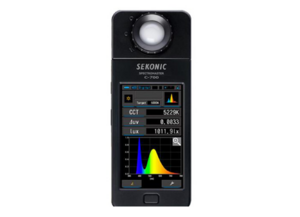
A spectrometer is used in ISP tuning to measure the color values of light sources accurately. It provides precise color data, which is essential for calibrating the ISP to achieve accurate color reproduction. It is mainly used to obtain the color temperature of the scene. Additionally, a luxmeter is mandatory to measure the light intensity of the scene for tuning purposes. Some devices combine both functions, allowing simultaneous measurement of color values and light intensity, which is essential for proper ISP tuning.

• Light box

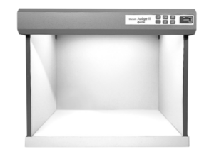
A light box is used in ISP tuning to provide a consistent and controlled lighting environment, ensuring uniform illumination for accurate color and exposure calibration. It helps eliminate external lighting variables, enabling precise adjustments. The light box should provide at least three different illuminants that closely simulate real-world lighting conditions. Additionally, its brightness must be adjustable to offer different illumination levels, typically around 1000 lux and 250 lux, to support tuning across various lighting intensities.

4.3. Tuning step by step

To execute the tuning procedure, start from a blank page:

1. Click on the "Start tuning from scratch" button to begin with a blank configuration of the ISP.

4.3.1. Step 1: Configure the statistics removal

Description:
This module removes potential statistical data inserted by a sensor before starting the demosaicing process, which could be affected by remaining statistics. It is typically used with sensors that have a parallel interface and cannot differentiate between statistics and pixel data. In contrast, CSI-2 sensors usually separate these data streams using different virtual channel IDs.

Configuration procedure:

1. Enable or disable the statistic removal module.
2. When enabled, you can configure the number of first lines to skip and the number of lines to keep. These parameters depend on the sensor datasheet.
3. Apply the configuration.

Information

With IMX335 sensor (this current example) the statistic removal is disabled. It is often the case with CSI-2 sensor

4.3.2. Step 2: Configure the bad pixel

Description:
This module aims to detect and correct artifacts generated by bad pixels on the sensor array. It is based on correlation extraction, not on fixed locations.
It works for RAW Bayer flows only, as RGB flows are assumed to be already cleaned.
All arriving components are scanned, and the horizontal continuity correlation with the two left and two right neighbors, on both the local component and the adjacent RAW Bayer component, is extracted:

• If a component is considered too light, it is declared bad.
• Components that are too dark are not extracted to avoid false positives.

If a component is assumed to be bad, it is replaced by the horizontal average of its two neighbors (with the same component).
When the module is enabled, the user can configure the strength from 0 (high tolerance) to 7 (aggressive detection). In return, the 12-bit counter reports the number of bad components corrected. The counter resets every frame.

Important

A bad pixel software algorithm has been implemented by STMicroelectronics. This algorithm takes as input a maximum number of pixels that the user might expect to detect; This is the threshold. The algorithm then updates the strength value of the bad pixel module to keep the amount of bad pixels detected close to the desired threshold.

Configuration procedure:

1. Enable the bad pixel module.
2. Once enabled, enable or disable the bad pixel software algorithm.
3. If the bad pixel algorithm is enabled, you can configure the threshold and in return be informed of the strength selected by the algorithm and the number of bad pixels detected. If the bad pixel algorithm is disabled, you can choose a fixed strength and in return be informed of the number of bad pixels detected.
4. Apply the configuration.

Information

The current manufacturing processes for image sensors minimize or eliminate defective pixels. Additionally, some image sensors feature automatic defective pixel correction, reducing the need for the ISP bad pixel module. We advise disabling this module if no bad pixel artifacts are detected.

4.3.3. Step 3: Configure the black level

Description:
This module suppresses a potential positive black-level offset, which occurs when the sensor sends non-null pixels while capturing a black picture. R, G, and B component offsets are subtracted from the R, G, and B Bayer components to achieve a black picture: R = G = B = 0.

Information

Most of the time, the black-level offset information can be found in the datasheet of the sensor. The following procedure can be used if this information is missing or to confirm it.

Configuration procedure:

1. Enable the black level module
2. Place a cap on the sensor (the preview frame is now black)
3. Open in the "Pixel Luminance" panel
4. Click on "Before demosaicing" to get the statistics before the demosaicing (in the RAW world)
5. Click on "Recalculate stats"
6. The "Average value of RGB & Luminance" graph is updated with the R, G, and B component averages that correspond to the black offset to be applied for each R, G, and B component. In this example, with the IMX335, we obtain R=12, G=12, and B=12.
7. Set the R, G, and B offset values
8. Apply the values by clicking the play button

Important

If obscuring the lens does not allow you to reach a totally black image, you can additionally set the sensor exposure time to its minimum

Information

Multiple offset values can be tested by adding a new configuration using the "Add new Offset" button. To select the configuration, click the play button. The applied configuration appears highlighted in blue.

4.3.4. Step 4: Configure the demosaicing

Description:
The module operates on the pixel pipes. It implements a medium-quality conversion from RAW Bayer 8 bpp to RGB 24 bpp. The output RGB pixel rate matches the input component rate.
The demosaicing process takes the surrounding 3x3 components as input, applies linear heuristics to determine the most likely missing components, and generates an output RGB888 pixel. The underlying heuristic filters try to extract and adapt to edges, horizontal and vertical lines, and lone pixels (0: no detection, pure linear interpolation; 1 to 7: relative detection strength).

Configuration procedure:

1. Enable the demosaicing module.
2. Once enabled, you can update the strength of the filters used to detect edges, horizontal and vertical lines, and lone pixels. The default values provide good results.
3. Apply the configuration.

Information

The demosaicing "RAW config", "Bayer pattern", and "Color depth" are retrieved from the sensor information and are set automatically . If one of the parameters is incorrect, it is likely that the sensor driver does not provide the correct information.

4.3.5. Step 5: Configure the gamma correction

Description:
This module implements a gamma compression on each R, G, and B component using a static gamma exponent of 2.2 to store gamma-compressed pictures, as defined in the sRGB standard.

Information

To achieve good color rendering while dumping the buffer, it is important to enable gamma on both pipe1 and pipe2.

Configuration procedure:

1. Enable gamma correction for both pipe1 and pipe2

4.3.6. Step 6: Configure the exposure control

Description:
This module aims to configure the sensor exposure to ensure the frame is well-exposed (neither too dark nor too bright). The exposure is not controlled by a parameter inside the ISP but by the sensor itself by updating the exposure time or the sensor gain, or both.

The user has the possibility to:

• Control the exposure manually by updating the gain or the exposure time, or both
• Enable the auto exposure algorithm
  • The algorithm automatically sets the appropriate sensor gain and exposure time based on statistics retrieved by the ISP and the ideal exposure target.
  • In this configuration, the user can control only the exposure compensation to shift the exposure target value and the anti-flicker mode.
• Configure the sensor delay parameter
• Read the estimated lux value of the scene

Information

The exposure compensation is expressed in exposure value (EV). +1EV doubles the exposure target -1EV halves the exposure target

Information

The sensor delay is the the number of frames needed by the sensor to reflect the sensor gain/exposure configuration. It can be set manually or can be automatically computed using the magic wand. The sensor delay can vary depending on the sensor frame rate. A sensor delay that is too long can cause latency in applying new parameters after the AE algorithm processing, while an incorrect sensor delay will inevitably lead to the algorithm malfunctioning.

Configuration procedure:

1. Enable the auto exposure algorithm (this does not impact the auto-calibration procedure)
2. If sensor delay feature is displayed, click on the magic wand to compute the sensor delay
3. Make sure the statistic are covers the entire color checker
4. The lux estimation and AE algorithm require parameter tuning for the lux calibration setup. This setup contains reference values essential for processing lux estimation and the AE algorithm, so tuning is mandatory.
   To perform this, you will need a light box with adjustable brightness and a lux meter. Then, you can either launch the auto-calibration procedure or manually tune the settings.

Information

To configure the statistics area, click on the Live Feedback picture and drag the mouse to draw the statistics area. The statistics region coordinates are then updated and the red dashed rectangle is displayed on the Live Feedback picture as well as on the preview in the LCD display. The color of the statistics area can be changed by clicking on the button above the Live Feedback picture. Possible values are: Default, Light, or Dark.

4.3.6.1. Auto-calibration procedure

The lux references are global sensor exposure values and luminance statistics collected under high lux conditions (preferably around 1000 lux) and low lux conditions (preferably around 250 lux).

4.3.6.1.1. Calibration of high lux references

1. Launch the auto-calibrate function to start the tuning.
2. In your lightbox, adjust the brightness to about 1000 lux. Then use a lux meter aimed at the color checker to measure the exact lux value received by the camera sensor. Enter this measured value in the "High lux target" field.
3. Next, start the calibration for high lux conditions

4.3.6.1.2. Calibration of low lux references

1. Calibration is paused because an action by the user is required
2. In your lightbox, adjust the brightness to about 250 lux. Then use a lux meter aimed at the color checker to measure the exact lux value. Enter this measured value in the "Low lux target" field.
3. Next, continue the calibration for low lux conditions
4. Once done, the new settings are applied automatically. You can save the tuning to exit the calibration setup.

Manual calibration procedure

4.3.6.2. Manual calibration procedure 4.3.6.2.1. Calibration of high lux references Disable the auto-exposure algorithm and adjust the brightness to about 1000 lux in your light box. Set the statistic area to cover the entire color checker. Then use a lux meter aimed at the color checker to measure the exact lux value. Adjust the sensor exposure to reach the luminance target of approximately 28 (−1EV). Record the global exposure time, the exact corresponding luminance, and the measured lux value. Then adjust the sensor exposure again to reach the luminance target of approximately 112 (+1EV). If the maximum exposure time is reached but you still need to increase exposure to reach the luminance target, you will also need to adjust the sensor gain. Then record this new global exposure time and the exact corresponding luminance. Open the Lux Calibration Setup window and set all the recorded values for high lux conditions (Sensor calibration factor must be 1 at this stage) Then save and apply these new settings. Enable the auto exposure algorithm Record the lux estimation computed by the tool. Get back to the Lux Calibration Setup window and enter the calibration factor calculated by the ratio between the lux estimation and the measured lux value: Then save and apply these new settings. Important The lux reference uses only global exposure time values. To compute these values, apply the following formula: 4.3.6.2.2. Calibration of low lux references Disable the auto-exposure algorithm and adjust the brightness to about 250 lux in your light box. Set the statistic area to cover the entire color checker. Then use a lux meter aimed at the color checker to measure the exact lux value. Adjust the sensor exposure to reach the luminance target of approximately 19 (−3/2EV). Record the global exposure time, the exact corresponding luminance, and the measured lux value. Then adjust the sensor exposure again to reach the luminance target of approximately 79(+1/2EV). If the maximum exposure time is reached but you still need to increase exposure to reach the luminance target, you will also need to adjust the sensor gain. Then record this new global exposure time and the exact corresponding luminance. Open the Lux Calibration Setup window and set all the recorded values for low lux conditions (Previous references for high lux are still set) Then save and apply these new settings. Enable the auto exposure algorithm Record the lux estimation computed by the tool. Get back to the Lux Calibration Setup window and enter the calibration factor obtained by calculating the average value between the high lux calibration factor and the low lux calibration factor: Then save and apply these new settings. Now, you can re-enable auto exposure algorithm and expect it to function properly. Important The tool provides real time estimation metrics. Lux estimation can be performed even when the AE algorithm is not running. However, it is mandatory to tune the Luxref configuration to obtain an accurate estimation.

Information

The auto exposure will adapt the sensor gain and exposure values during the auto white balance profile calibration. Therefore, it needs to be enabled prior to the AWB tuning procedure.

4.3.7. Step 7: Configure auto white balance (AWB) profiles

Information

In the following description of the AWB profile configuration, a white balance profile for a given illuminant refers to a combination of several sets of parameters: a color temperature, the ISP gains associated with a color correction matrix (CCM) and the raw RGB statistics of the profile.

Important

A maximum of 5 different white balance profiles are supported by the auto white balance algorithm. However, at least 3 profiles are needed for the AWB to provide accurate results. These recommended profiles should have color temperatures around 2500, 4000, and 6500 kelvin.

Description:
This module interacts with the ISP gains and the color correction matrix block:

• The ISP gain equalizes the R, G, and B components by applying independent gains to each R, G, and B component to ensure white appears white.
• The color correction matrix converts the frame from the sensor RGB space to the sRGB space to achieve good color rendering.

Configuration procedure:
To perform the tuning of each profile, you will need a light box with at least three different illuminants. Start by setting an illuminant. Then, you can either launch the auto-calibration procedure or manually tune the settings.

4.3.7.1. Auto-calibration procedure

4.3.7.1.1. Auto-calibrate WB profile

1. Enable the white balance correction module and ensure that the AWB algorithm is disabled.
2. Create a new white balance profile. Newly created profiles always have all gains set to 1 and a CCM set with an identity matrix.
3. Name your profile and set the color temperature information box with the value retrieved using the spectrometer.
4. Apply the white balance profile.
5. In the menu, select "Auto calibrate".
6. The color checker is detected automatically. But if you have moved the color checker in your scene, you can refresh the image and restart the automatic detection.
7. Set the target temperature with the measured color temperature.
8. Additionally, if the color checker area is not a rectangle, you can adjust each corner to better fit the color checker in the image.
9. Then start calibration of the profile (the processing may take a few minutes)
10. Once the calibration is complete, you can drag the vertical slider to compare each patch of the color checker before and after correction.
11. If the result is good, apply and save the new tuning parameters. If it does not seem good, you can relaunch the procedure with "Try Again" button.

Information

At this stage, the color rendering for the selected illuminant is close to the reference.

4.3.7.1.2. Analyze the final ISP configuration to check color accuracy versus the reference colors

1. Make sure the profile you want to analyze is correctly applied.
2. Then take an RGB picture of the color checker with ISP gain and CCM applied (frame is saved as a .png file).
3. Open the "Analysis" panel.
4. Select "Advanced Image" analysis.
5. Upload the RGB picture (.png file).
6. Start the advanced image analysis.
7. The color analysis is complete, and you can verify the color accuracy with the different graph and information provided.
8. Optionally, you can download the analysis results as a zip file containing the graphs and .csv file.

Information

The color analysis provides information and metrics on how the colors are rendered according to the ISP configuration: DeltaE00 (ΔE00): color difference metric based on the CIEDE2000 formula measuring the overall color difference, including lightness, chroma, and hue. ΔE00 is informative, acceptance criteria is based on ΔC00 (see below) DeltaC00 (ΔC00): color difference metric based on the CIEDE2000 formula measuring only the chroma difference, ignoring lightness and hue differences. ΔC00 neutral gray patches acceptance criteria: ΔC00 < 5 ΔC00 other patches acceptance criteria: ΔC00 < 10 R/G and B/G ratio: neutrality of the gray patches in a color checker. For a neutral gray patch, the ideal ratios should be close to 1:1, indicating that the red, green, and blue channels are balanced, resulting in a neutral gray color. R/G ratio acceptance criteria: typically between 0.9 and 1.1 B/G ratio acceptance criteria: typically between 0.9 and 1.1 Exposure error: refers to the deviation of an image's exposure from the ideal exposure level. When using color checker charts, the reference color values are only accurate if the exposure is correct. Exposure error acceptance criteria: ± 0.250 f-stop If exposure error is not in the acceptance criteria, the sensor exposure needs to be increased or decreased accordingly. Description of the graph results: 3D bar graph representing the ΔC00 value of each patch compared to the reference value. A low bar indicates better color accuracy. Mean and max ΔE00 and ΔC00 are also provided. Graph providing information about the neutral gray patches: The top graph represents the log pixel level of each component (R, G, B) versus the neutral gray patch density. R, G, and B curves must be as close as possible for a good neutral gray patch rendering. This graph also provides the exposure error value and the measured value of the gamma. The bottom graph represents the ΔC00 versus the neutral gray patch density. Note: Density represents the extent to which light is absorbed. Visual representation of the ISP color rendering compared to the reference value (ISP color rendering is represented by the square in the middle of the reference color). .csv file with the complete data that permit to draw the graphs A, B, and C.

Manual calibration procedure

4.3.7.2. Manual calibration procedure 4.3.7.2.1. Configure the ISP gain to ensure white appears white Enable the white balance correction module and ensure that the AWB algorithm is disabled. Create a new white balance profile. Newly created profiles always have all gains set to 1 and a CCM set with an identity matrix. Name your profile and set the color temperature information box with the value retrieved using the spectrometer. Apply the white balance profile. Set the statistics area to cover the entire color checker. Take a RAW Bayer picture of the color checker (picture is saved as a .pgm file). Open the "Analysis" panel. Select "White Balance Gain" analysis. Upload the RAW Bayer picture (.pgm file). Start the white balance gain analysis. If the analysis fails, it is likely that the color checker is not detected because it is underexposed. In that case, slightly update the sensor exposure time and perform the steps again from step 1. Get the R, G, and B ISP gains computed by the analysis tool. Go back to the "White Balance" panel and set the R, G, and B gains of your white balance profile. Apply the white balance profile. Once done, take an RGB picture of the color checker with ISP gain applied (frame is saved as a .png file) for the next step. 4.3.7.2.2. Configure the color correction matrix for optimal color rendering Open the "Analysis" panel. Select "Color Correction Matrix" analysis. Upload the RGB picture (.png file) Start the CCM analysis. Get the CCM coefficient that have been computed (you can use the copy button to save those values). Go back to the "White Balance" panel and edit the CCM coefficients. Paste the coefficient values that have been copied (or you can fill the matrix manually) Save the new CCM. Important Before applying the new coefficients of the CCM, verify that the CCM coefficients correspond to the identity matrix. If the CCM coefficients do not correspond to the identity matrix before applying the new coefficients, it is likely that you performed the CCM analysis based on a non-identity matrix, which will lead to an incorrect final color. 4.3.7.2.3. Collect the RAW RGB statistics of the profile Open RGB statistics menu. Click on "Collect RGB stats" to update the statistics of the current profile Save this data collection Important It is really important to collect properly the raw RGB statistics (before demosaicing) of the profile. Otherwise, the AWB algorithm will not be set properly and you will get the following warning message: 4.3.7.2.4. Analyze the final ISP configuration to check color accuracy versus the reference colors Once the profile is tuned and applied, analyze the final image using the analysis procedure described above.

4.3.7.3. Enable the AWB algorithm

Once you have at least 3 tuned profiles, you will be able to launch the AWB algorithm.

1. Select the white balance profile to be managed by the AWB algorithm.
2. Activate the AWB algorithm.

Information

The yellow tick box turns into the AWB logo when AWB is active. When AWB is active, the profile selected by the AWB algorithm is highlighted in blue.

Information

In case of RGB sensor, it is advised to relaunch this calibration procedure after AWB tuning procedure since the color correction might change the statistics measurements.

4.3.8. Step 8: Configure the contrast (optional)

Description:
This module concludes the image processing pipeline. It enhances the contrast of the frame by non-linear emphasis of pixel luminance. It takes the RGB values from the pipeline, computes the luminance of the local pixel, and determines the desired luminance adjustment factor based on the input luminance using a lookup table. The output RGB components are clamped to 8 bits.

Configuration procedure:

1. Enable the contrast module
2. Select a predefined contrast profile
3. Optionally tune the LUT
4. Apply the contrast settings

4.3.9. Step 9: Export the ISP configuration

Description:
Once the ISP tuning is finalized, the ISP configuration needs to be exported so that the ISP settings and behaviors are reflected in the final application.

Configuration procedure:

1. Open the "My Configuration" panel
2. Click on "Export Configuration" and chose the export format suitable for your project:
   1. For a Linux project, you need to export the ISP configuration as a .yaml file.
   2. For a bare-metal MCU project, you need to export the ISP configuration as a .h code file.

Information

Linux: The generated .yaml file must be uploaded to the target in the following directory: scp <sensor .yaml file> root@<IP address of the platform>:/usr/share/libcamera/ipa/dcmipp/ The selection of the .yaml file is done at runtime based on the name of the detected sensor. If the name of the detected sensor is imx335, then the imx335.yaml file is loaded by libcamera to set the ISP configuration created by the user.

Information

Bare-metal MCU: The isp_param_conf.h generated file must be copied in the application project to take into account the ISP configuration created by the user.

4.4. Tips

4.4.1. Save and load your current work

4.4.2. Load a saved work

4.4.3. Sensor information at a glance

All the sensor information is summarized in the "Sensor Information" panel.

4.4.4. Current configuration at a glance

All ISP module status is summarized in the "My Configuration" panel.