This document presents several use case studies where NanoEdge AI Studio has been used successfully to create smart devices with machine learning features using a NanoEdge AI library.
The aim of the document is to explain the methodology and thought process behind the choice of crucial parameters during the initial datalogging phase (that is, even before starting to use NanoEdge AI Studio) that can make or break a project.
For each use case, the focus is on the following aspects:
- what is a meaningful representation of the physical phenomenon being observed
- how to select the optimal sampling frequency for the datalogger
- how to select the optimal buffer size for the data sampled
- how to format the data logged properly for the Studio
Details about hardware and code implementation are irrelevant here and not discussed in this article.
Recommended: NanoEdge AI Datalogging MOOC. This eLearning course contains all relevant information about the whole datalogging pipeline for NanoEdge AI, from simple datalogger creation using STM32CubeIDE, to library implementation. These are both for anomaly detection and classification projects, with in-depth explanations and several code examples.
Refer to the NanoEdge AI documentation for more information.
1. Summary of important concepts
1.1. Definitions
Here are some clarifications regarding important terms that are used in this document:
- "axis/axes": total number of variables outputted by a given sensor. Example: a 3-axis accelerometer outputs a 3-variable sample (x,y,z) corresponding to the instantaneous acceleration measured in 3 perpendicular directions.
- "sample": this refers to the instantaneous output of a sensor, and contains as many numerical values as the sensor has axes. For example, a 3-axis accelerometer outputs 3 numerical values per sample, while a current sensor (1-axis) outputs only 1 numerical value per sample.
- "signal", "signal example", or "learning example": used interchangeably, these refer to a collection of numerical values that are used as input in the NanoEdge AI functions, either for learning of for inference. The term "line" is also used to refer to a signal example, because in the input files for the Studio, each line represents an independent signal example.
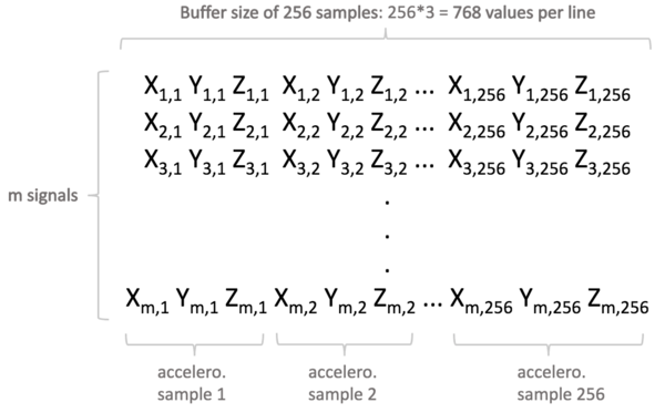
- "buffer size", or "buffer length"; this is the number of samples per signal. It must be a power of 2. For example, a 3-axis signal with buffer length 256 is represented by 768 (256*3) numerical values.
1.2. Sampling frequency
The sampling frequency, sometimes referred to as (output) data rate, corresponds to the number of samples measured per second.
The speed at which the samples are taken must allow the signal to be accurately described, or "reconstructed". The sampling frequency must be high enough to account for the rapid variations of the signal. The question of choosing the sampling frequency therefore naturally arises:
- If the sampling frequency is too low, the readings are too far apart. If the signal contains relevant features between two samples, they are lost.
- If the sampling frequency is too high, it may negatively impact the costs, in terms of processing power, transmission capacity, or storage space for example.
The issues related to the choice of sampling frequency and the number of samples are illustrated below:
- Case 1: the sampling frequency and the number of samples make it possible to reproduce the variations of the signal.

- Case 2: the sampling frequency is not sufficient to reproduce the variations of the signal.

- Case 3: the sampling frequency is sufficient but the number of samples is not sufficient to reproduce the entire signal (meaning that only part of the input signal is reproduced).

1.3. Buffer size
The buffer size corresponds to the total number of samples recorded per signal, per axis. In the case of a temporal signal, the sampling frequency and the buffer size put a constraint on the effective signal temporal length.
The buffer size must be a power of 2.
The buffer length must be chosen carefully, depending on the characteristics of the physical phenomenon sampled. For instance, the buffer may be chosen to be as short as a few periods in the case of a periodic signal (such as current, or stationary vibrations). In other cases, for instance when the signal is not purely periodic, the buffer size can be chosen to be as long as a complete operational cycle of the target machine to monitor (example: a robotic arm that moves from point A to point B, or a motor that ramps up from speed 1 to speed 2, and so on).
In some cases, where the signal considered is not temporal (example: time-of-flight sensor), the buffer size is simply constrained by the size and resolution of the sensor's output (for instance, a buffer size of 64 for a 8x8 time-of-flight array).
1.4. Data format
In the Studio, each signal is represented by an independent line, which format is completely constrained by the chosen buffer length and sampling frequency.
Example:
Here is the input file format for a 3-axis sensor (in this example, an accelerometer), where the buffer size chosen is 256. Let's consider that the sampling frequency chosen is 1024 Hz. It means that each line (here, "m" lines in total) represents a temporal signal of 256/1024 = 250 milliseconds.
In summary, this input file contains "m" signal examples representing 250-millisecond slices of the vibration pattern the accelerometer is monitoring.
2. Use case studies
2.1. Vibration patterns on a ukulele
2.1.1. Context and objective
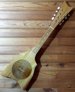
In this project, the goal is to capture the vibrations produced when the ukulele is strummed, in order to classify them, based on which individual musical note, or which chord (superposition of up to 4 notes), is played.
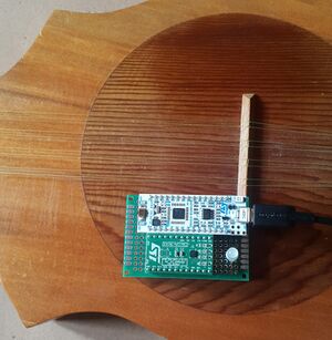
This is achieved using vibration (3-axis accelerometer) instead of sound (microphone). The 3-axis accelerometer is placed directly onto the ukulele, or in the sounding box, wherever the vibrations are expected to be most intense.
In this application, the signals used are temporal.
2.1.2. Initial thoughts
Even before starting data collection, it is necessary to analyze the use case, and think about the characteristics of the signal we are about to sample. Indeed, we want to make sure that we capture the essence of the physical phenomenon that takes place, in a way that it is mathematically meaningful for the Studio (that is, making sure the signal captured contains as much useful information as possible).
When strumming the ukulele, some important characteristics of the vibration produced can be noted:
- The action of strumming is sudden. Therefore the signal created is a burst of vibration, and dies off after a couple of seconds. The vibration may be continuous on a short time scale, but it does not last long, and is not periodic on a medium or long time scale. This is helpful to determine when to start signal acquisition.
- The previous observation is also useful to choose a proper buffer size (how long the signals should be, or how long the signal capture should take).
- The frequencies involved in the vibration produced are clearly defined, and can be identified through the pitch of the sound produced. This is helpful to determine the target sampling frequency (output data rate) of the accelerometer.
- The intensity of the vibrations are somewhat low, therefore we have to be careful about where to place the accelerometer on the ukulele's body, and how to choose the accelerometer's sensitivity.
2.1.3. Sampling frequency
When strumming the ukulele, all the strings vibrate at the same time, which makes the ukulele itself vibrate. This produces the sound that we hear, so we can assume that the sound frequencies, and the ukulele vibration frequencies, are closely related.
Each chord contains a superposition of four musical notes, or pitches. This means we have four fundamental frequencies (or base notes) plus all the harmonics (which give the instrument its particular sound). These notes are quite high-pitched, compared to a piano for example. For reference, we humans can usually hear frequencies between 20 Hz and 20000 Hz, and that the note A (or la) usually has a fundamental frequency of 440 Hz. Thus, we can estimate that the chords played on the ukulele contain notes between 1000 Hertz and 10000 Hertz maximum.
To be more precise, and learn more about our signal, we can use a simple real-time frequency analyzer. In this example, we are using Spectroid, a free Android application.
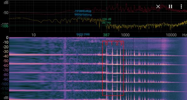
Here is the spectrogram obtained when playing the C major chord (or do) several times.
Here's the spectrogram on a F major chord (fa).
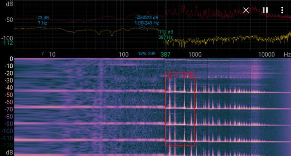
In both cases, the fundamental frequency (0) and the 3 first harmonics (1, 2, 3) are between around 380 Hz and 1000 Hz. There are many more harmonics up to 10 kHz, but they rapidly decrease in intensity, so we can assume for the moment that 1000 Hz is the maximum frequency to sample.
To perform this, we need to set the sampling frequency to at least double that frequency; 2000 Hz minimum.
In this example, the accelerometer used only supports a discrete range of sampling frequencies, among which: 1666 Hz, 3333 Hz and 6666 Hz.
We start testing with a sampling frequency of 3333 Hz. We adapt later, depending on the results we get from the Studio, for instance by doubling the frequency to 6666 Hz for more precision.
2.1.4. Buffer size
The buffer size is the number of samples that compose our vibration signal.
When strumming the ukulele, the sound produced lasts for one second or so. The vibration on the ukulele body quickly dies off. Therefor we can assume that capturing a signal of maximum 0.5 seconds is enough. We adapt later, depending on the results we get from the Studio.
With a target length of approximately 0.5 seconds, and a sampling frequency of 3333 Hz, we get a target buffer size of 3333*0.5 = 1666.
The chosen buffer size must be **a power of two**, let's go with 1024 instead of 1665. We can have picked 2048, but 1024 samples is enough for a first test. We can always increase it later if required.
As a result, the sampling frequency of 3333 Hz with the buffer size of 1024 (samples per signal per axis) make a recorded signal length of 1024/3333 = 0.3 seconds approximately.
So each signal example that is used for data logging, or passed to a NanoEdge AI function for learning or inference, represent a 300-millisecond slice of vibration pattern. During these 300 ms, all 1024 samples are recorded continuously. But since all signal examples are independent from one another, whatever happens between two consecutive signals does not matter (signal examples do not have to be recorded at precise time intervals, or continuously).
2.1.5. Sensitivity
The accelerometer used supports accelerations ranging from 2g up to 16g. For gentle ukulele strumming, 2g or 4g are enough (we can always adjust it later).
We choose a sensitivity of 4g.
2.1.6. Signal capture
In order to create our signals, we can imagine continually recording accelerometer data. However, we chose an actual signal length of 0.3 seconds. So if we started strumming the ukulele randomly, using continuous signal acquisition, we then end up with 0.3-second signal slices that do not necessarily contain the useful part of the strumming, and have no guarantee that the relevant signals are captured. Also, a lot of "silence" would be recorded, between strums.
Instead, we implement a trigger mechanism; so that only the vibration signature that directly follows a strum is recorded.
Here are a few ideas on how to implement such a trigger mechanism that detects a strum:
- We want to the capture of a single signal buffer (1024 samples) whenever the intensity of the ukulele's vibrations cross a threshold.
- We need to monitor the vibrations continuously, and check whether or not the intensity has suddenly risen.
- To measure the average vibration intensity at any time, we collect very small data buffers from the accelerometer (example: 4 consecutive samples), and compute the average vibration intensity across all sensor axes for each such "small buffer".
- We continuously compare the average vibration intensities obtained from one "small buffer" (let's call it I1) to the next (call it I2).
- We choose a threshold (example: 50%) to decide when to trigger (here, for instance, whenever I2 is at least 50% higher than I1).
- We trigger the recording of a full 1024 sample signal buffer whenever I2 >= 1.5*I1 (here using 50%).
The resulting 1024-sample buffer is used as input signal in the Studio, and later on in the final device, as argument to the NanoEdge AI learning and inference functions.
Of course, different approaches (equivalent, or more elaborate) might be used in order to get a clean signal.
Here is what the signal obtained after strumming one chord on the ukulele looks like (plot of intensity (g) vs. time (sample number), representing the accelerometer's x-axis only):
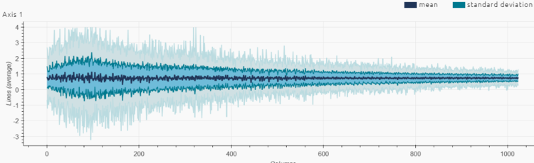
Observations:
- There is no saturation/clipping on the signal (y-axis of the plot above), so the sensitivity chosen for the accelerometer seems right.
- The length seems appropriate because it is much longer than a few periods of all the frequency components contained in our vibration, and therefore contains enough information.
- The length also seems appropriate because it represents well the vibration burst associated to the strumming, including the quick rise and the slower decay.
- If the signal needs to be shortened (for instance, if we need to limit the amount of RAM consumed in the final application), we can consider cutting it in half (truncating it after the first 512 samples), and the resulting signal would probably still be very usable.
- The number of numerical values in the signal shown here is 1024 because we're only showing the x-axis of the accelerometer. In reality, the input signal is composed of 1024*3 = 3072 numerical values per signal.
2.1.7. From signals to input files
Now that we managed to get a seemingly robust method to gather clean signals, we need to start logging some data, to constitute the datasets that are used as inputs in the Studio.
The goal is to be able to distinguish all main diatonic notes and chords of the C major scale (C, D, E, F, G, A, B, Cmaj, Dm, Em, Fmaj, G7, Am, Bdim) for a total of 14 individual classes.
For each class, we record 100 signal examples (100 individual strums). This represents a total of 1400 signal examples across all classes.
100 is an arbitrary number, but fits well within the guidelines: a bare minimum of 20 signal examples per sensor axis (here 20*3 = 60 minimum) and a maximum of 10000 (there is usually no point in using more than a few hundreds to a thousand learning examples).
When recording data for each class (example, strumming a Fmaj chord 100 times), we make sure to introduce some amount of variety: slightly different finger pressures, positions, strumming strength, strumming speed, strumming position on the neck, overall orientation of the ukulele, and so on. This increases the chances that the NanoEdge AI library obtained generalizes/performs well in different operating conditions.
Depending on the results obtained with the Studio, we adjust the number of signals used for input, if needed.
In summary:
- there are 14 input files in total, one for each class
- the input files contain 100 lines each
- each line in each file represents a single, independent "signal example"
- there is no relation whatsoever between one line and the next (they could be shuffled), other than the fact that they pertain to the same class
- each line is composed of 3072 numerical values (3*1024) (3 axes, buffer size of 1024)
- each signal example represents a 300-millisecond temporal slice of the vibration pattern on the ukulele
2.1.8. Results
Here are the benchmark results obtained in the Studio, with 14 classes, representing all main diatonic notes and chords of the C major scale.
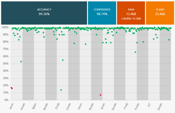
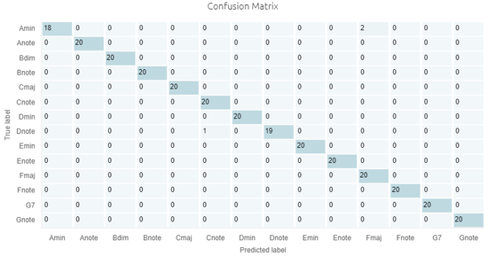
Here are the performances of the best classification library, summarized by its confusion matrix:
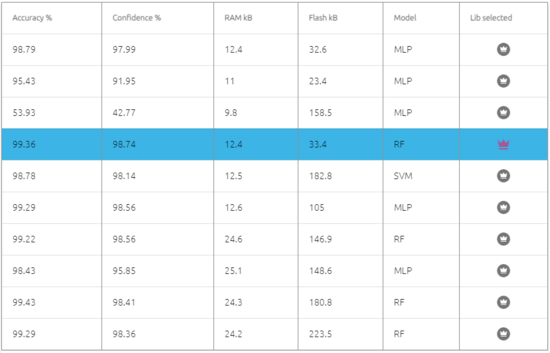
Here are some other candidate libraries that were found during benchmark, with their associated performances, memory footprint, and ML model info.
Observations:
- We get excellent results with very few misclassifications.
- There is no need to adjust the datalogging settings.
- We can consider adjusting the size of the signal (taking 512 samples instead of 1024) to reduce the memory footprint (RAM) of the libraries.
- Before deploying the library, we can do additional testing, by collecting more signal examples, and running them through the NanoEdge AI Emulator, to check that our library indeed performs as expected.
- If collecting more signal examples is impossible, we can restart a new benchmark using only 60% of the data, and keep the remaining 40% exclusively for testing using the Emulator.
2.2. Static pattern recognition (rock, paper, scissors) using time-of-flight
2.2.1. Context and objective
In this project, the goal is to use a time-of-flight sensor to capture static hand patterns, and classify them depending on which category they belong to.
The three patterns that are recognized here are: "Rock, Paper, Scissors", which correspond to 3 distinct hand positions, typically used during a "Rock paper scissors" game.

This is achieved using a time-of-flight sensor, by measuring the distances between the sensor and the hand, using a square array of size 8x8.
2.2.2. Initial thoughts
In this application, the signals used are not temporal.
Only the shape/distance of the hand is measured, not its movement.
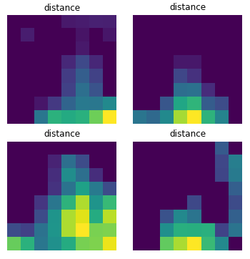
Here is an illustration of four independent examples of outputs from the time-of flight sensor. The coordinates of each measuring pixel is translated by its position on the 2D array, and the color of each pixel translates how close to the sensor the object is (the brighter the pixel, the closer the hand).
2.2.3. Sampling frequency
Because each signal is time-independent, the choice of a sampling frequency is irrelevant to the structure of our signals. Indeed, what we here consider as a full "signal" is nothing more than a single sample; a 8x8 array of data, in the form of 64 numerical values.
However, we choose a sampling frequency of 15 Hz, meaning that a full signal is to be outputted every 1/15th of a second.
2.2.4. Buffer size
The size of the signal is already constrained by the size of the sensor's array.
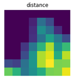
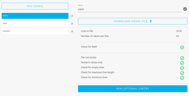
As mentioned above, each "signal example" used as input in the Studio is a single 8x8 array, as shown above. In practice, each array is represented as a line composed of 64 numerical values representing distances in millimeters. For example:
96.0 93.0 96.0 90.0 105.0 98.0 101.0 0.0 93.0 96.0 98.0 94.0 105.0 98.0 96.0 0.0 97.0 98.0 98.0 96.0 104.0 98.0 96.0 0.0 97.0 99.0 97.0 94.0 104.0 100.0 96.0 0.0 100. 0 98.0 96.0 96.0 103.0 98.0 98.0 0.0 99.0 97.0 98.0 97.0 102.0 98.0 101.0 0.0 102.0 99.0 100.0 100.0 102.0 98.0 102.0 0.0 102.0 95.0 99.0 96.0 96.0 96.0 102.0 102.0
2.2.5. Signal capture
In order to create our signals, we can imagine continually recording time-of-flight arrays. However, it is be preferable to do so only when needed (that is, only when some movement is detected under the sensor). This is also useful after the datalogging phase is over, when we implement the NanoEdge AI Library; inferences (classifications) only happen after some movement has been detected.
So instead of continuous monitoring, we use a trigger mechanism that only starts recording signals (arrays, buffers) when movement is detected. Here, it is built-in to the time-of-flight sensor, but it could easily be programmed manually. For instance:
- Choose threshold values for the minimum maximum detection distances
- Continuously monitor the distances contained in the 8x8 time-of-flight buffer
- Only keep a given buffer if at least 1 (or a predefined percentage) or the pixels returns a distance value comprised between the two predefined thresholds
During the datalogging, this approach prevents the collection of "useless" empty buffers (no hand). After the datalogging procedure (after the library is implemented), this approach is also useful to limit the number of inferences, effectively decreasing the computational load on the microcontroller, and its power consumption.
2.2.6. From signals to input files
The input signal is well defined, and needs to be captured in a relevant manner for what needs to be achieved.
The goal is to distinguish among three possible patterns, or classes. Therefore, we create three input files, each corresponding to one of the classes: rock, paper, scissors.
Each input file to contain a significant number of signal examples (~100 minimum), covering the whole range of "behaviors" or "variety" that pertain to a given class. For instance, for "stone", we need to provide examples of many different versions of "stone" hand positions, that describe the range of everything that could happen and rightfully be called "stone". In practice, this means capturing slightly different hand positions (offset along any of the two directions of the time-of-flight array, but also, at slightly different distances from the sensor), orientations (hand tilt), and shapes (variations in the way the gesture is performed).
This data collection process is greatly helped by the fact that we sample sensor arrays at 15 Hz, which means that we get 900 usable signals per minute.
For each class, we collect data in this way for approximately three minutes. During these three minutes, slight variations are made:
- to the hand's position in all 3 directions (up/down left/right, top/bottom)
- to the hand's orientation (tilt in three directions)
- to the gesture itself (example, for the "scissors" gesture, wiggle the two fingers slightly)
We get a total of 3250 signal examples for each class.
2.2.7. Results
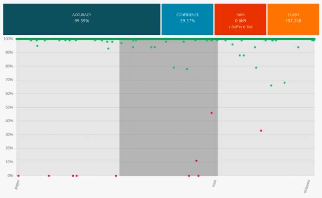
Below are the classification benchmark results obtained in the Studio with these three classes.
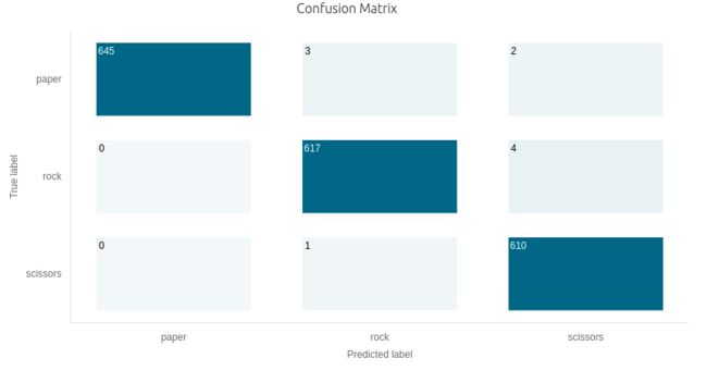
Here are the performances of the best classification library, summarized by its confusion matrix.
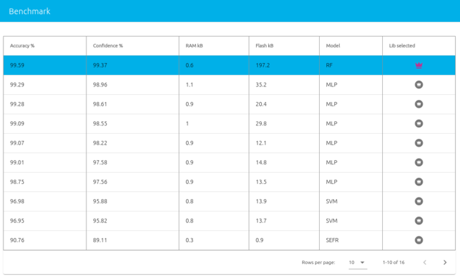
Below are some other candidate libraries that were found during benchmark, with their associated performances, memory footprint, and ML model info.
Observations:
- We get excellent results with very few misclassifications.
- Before deploying the library, it is good practice to test it by collecting more signal examples, and running them through the NanoEdge AI Emulator, to check that our library indeed performs as expected.
- Considering two libraries with similar performances (accuracy, confidence), experience shows that libraries requiring more flash memory often generalize better to unseen data (more reliable / adaptable when testing in slightly different conditions).
2.3. Dynamic people counting using Time-of-Flight
2.3.1. Context and objective
In this project, the goal is to use a time-of-flight sensor to capture people's movement while crossing a gate, and classify these movements into distinct categories. Here are some examples of behaviors to distinguish:
- One person coming in (IN_1)
- One person going out (OUT_1)
- Two people side-by-side coming in (IN_2)
- Two people side-by-side going out (OUT_2)
- Two people crossing the gate simultaneously in opposite directions (CROSS)
This is achieved using a time-of-flight sensor, by measuring the distances between the sensor (for example, mounted on the ceiling, or on top of the gate, looking down to the ground) and the people passing under it.
The time-of-flight arrays outputted by the sensor are 8x8 in resolution:
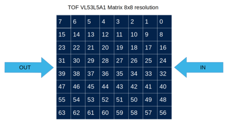
This device, placed at the entrance of a room, can also be used to determine the number of people present in the room.
2.3.2. Initial thoughts
In this application, because we want to capture movements and identify them, the signals considered have to be temporal.
This means that each signal example that are collected during datalogging, and that use later on to run inference (classification) using the NanoEdge AI library, have to contain several 8x8 arrays in a row. Putting several 8x8 sensor frames in a row enables us to capture the full length of person's movement.
Note: in order to prevent false detections (for example, a bug flying in front of the sensor, or pets / luggage crossing the sensor frame), we set on the sensor a minimum and maximum threshold distance.
#define MIN_THRESHOLD		100	/* Minimum distance between sensor & object to detect */
#define MAX_THRESHOLD		1400 	/* Maximum distance between sensor & object to detect */
2.3.3. Sampling frequency and buffer size
For the sampling frequency, we choose the maximum rate available on the sensor: 15 Hz.
The duration of a person's movement crossing the sensor frame is estimated to be about 2 seconds. To get a two-second signal buffer, we need to get 15*2 = 30 successive frames, as we sample at 15 Hz.
It is good practice to choose a power of two for buffer lengths, in case the NanoEdge AI library requires FFT pre-processing (this is determined automatically by the Studio during benchmarking), so we choose 32 instead of 30.
With 32 frames sampled at 15 Hz, it means each signal represents a temporal length of 32/15 = 2.13 seconds, and contains 32*64 = 2048 numerical values.
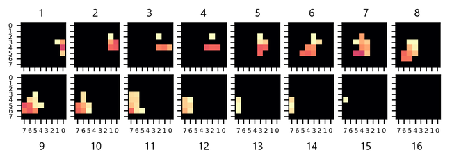
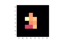
Below is a visual representation of a signal example, corresponding to one person coming in (moving from the right to the left of the frame).
Note: only half of the movement is represented, from frame 1 to frame 16 (the complete buffer has 32 frames). Red/purple pixels correspond to a presence detected at a short distance, yellowish pixels at a longer distance, and black pixels mean no presence detected (outside of the MIN_THRESHOLD and MAX_THRESHOLD).
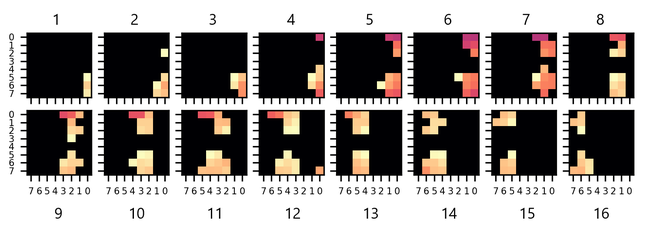
Here are two people coming in (moving from the right to the left of the frame):
And two people crossing (person at the top moving from right to left, person at the bottom moving from left to right):
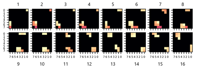
Note that some movements are faster than others: for some buffers, the last portion of the signal may be blank (empty / black frames). This is not necessarily a problem, instead it increases signal variety (as long as we also get other sorts of signals, some shorter, some longer, some offset, and so on), which can result in a more robust, more generalizable NanoEdge AI library.
2.3.4. Signal capture
Here, we won't collect ~2-second buffers continuously, but only when a presence is detected under the sensor. This presence detection is built-in to the time-of-flight sensor (but it could be easily re-coded, for example by monitoring each pixel, and watching for sudden changes in distances).
So as soon as some movement is detected under the sensor, a full 32-frame buffer is collected (2048 values).
We also want to prevent buffer collection whenever a static presence is detected under the sensor for an extended time period. To do so, a condition is implemented just after buffer collection, see below, in pseudo-code:
while (1) {
    if (presence) {
        collect_buffer();
        do {
            wait_ms(1000);
        } while (presence);
    }
}
2.3.5. From signals to input files
For this application, the goal is to distinguish among 5 classes:
- One person coming in (IN_1)
- One person going out (OUT_1)
- Two people side-by-side coming in (IN_2)
- Two people side-by-side going out (OUT_2)
- Two people crossing the gate simultaneously in opposite directions (CROSS)
We therefore create fives files, one for each class. Each input file is to contain a significant number of signal examples (~100 minimum), covering the whole range of "behaviors" or "variety" that pertain to a given class. This means that approximately 100 movements for each class must be logged (total of ~500 across all classes), which may be tedious, bus is nonetheless necessary.
With this base of 100 signal examples per class, a couple of additional steps can be carried out for better efficiency and performances: data binarization, and data augmentation.
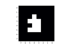
Data binarization:
In this application, the goal is to detect a movement and characterize it, not to measure distances. Therefore, in order to simplify the input data buffers as much as possible, we replace the distance values by binary values. In other words, whenever a pixel detects some amount of presence, the distance value is replaced with 1, otherwise, it is replaced with 0.
Data augmentation:
To enrich the data, and cover some corner cases (for example, a person passing not in the middle of the frame, but near the edge), we may artificially expand the data, for example using a Python script. Here are some examples of operation that could be made:
- shifting the pixel lines on each frame up or down incrementally, one pixel at a time: by doing this, we simulate datalogs where each movement is slightly offset spatially, up or down, on the sensor's frame. This is done, on the flat 2048-value buffer, by shifting 8-value pixel lines to the right, or to the left (by 8 places) for each 64-value frame, and repeating the operation on all 32 frames. The 8 blank spaces created in this way are filled with zeros.
- shifting the frames contained on each buffer: by doing this, we simulate datalogs where each movement is slightly offset temporally (each movement starts one frame sooner, or one frame later). This is done, on the flat 2048-value buffer, by shifting all 32 64-value frames, to the right, or to the left (by 64 places). The 64 blank spaces created in this way are filled with zeros.
- inverting the frames, so that one type of movement becomes its opposite (for example, "IN_1" would become "OUT_1"). The same can be done to create "OUT_2" by inverting the buffers logged from "IN_2". This would be achieved on the 2048-value buffer by reversing each 8-value pixel line (inverting the order of the 8 numerical values corresponding to a pixel line) for each 64-value frame, and repeating the operation for all 32 frames.
After data binarization and augmentation, we end up with approximately 500-1500 signal examples per class (number of signals per class don't have to be perfectly balanced). For example, we have 470 signals for the class "IN_2":
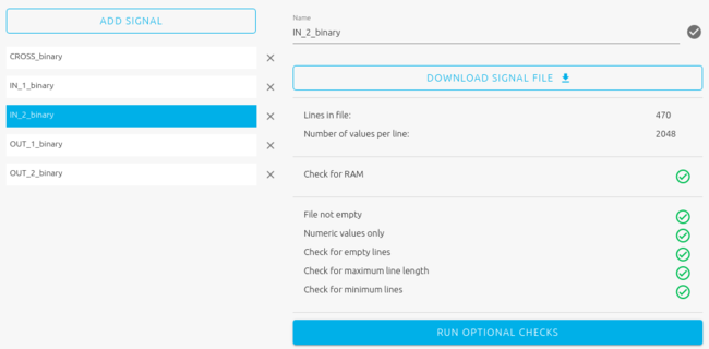
Here is the 2048-value signal preview for "IN_2":
2.3.6. Results
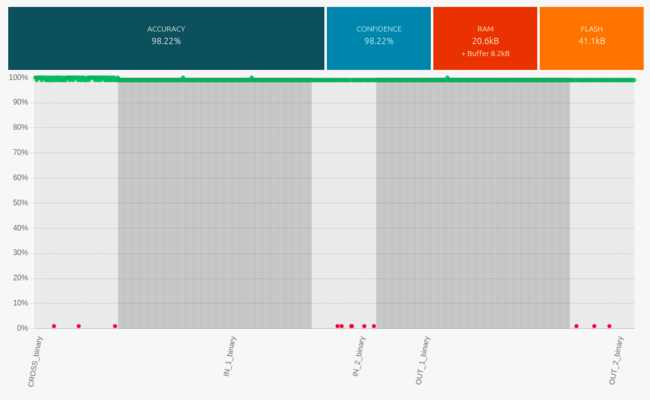
Here are the classification benchmark results obtained in the Studio with these 5 classes.
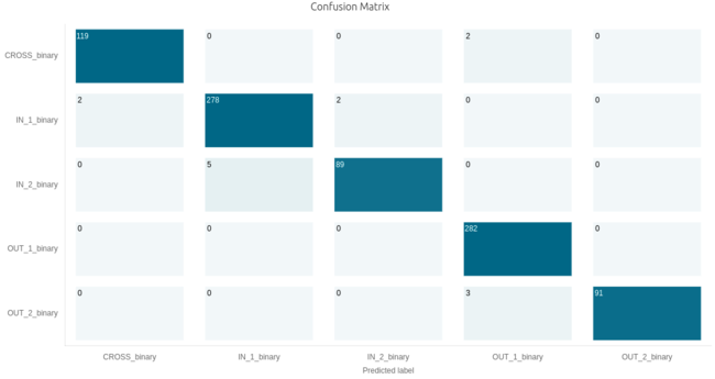
Here are the performances of the best classification library, summarized by its confusion matrix.
Here are some other candidate libraries that were found during benchmark, with their associated performances, memory footprint, and ML model info.
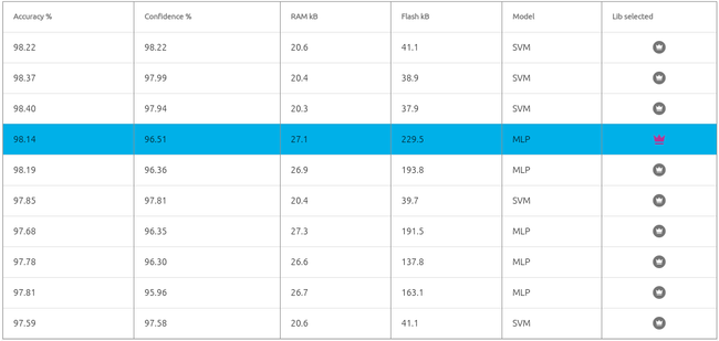
Note: on the picture above, the best library automatically selected by the Studio is displayed on the 1st line (SVM model, 41.1 KB flash). Here instead, we manually selected a different library (4th line, MLP model, 229.5 KB flash). Indeed, on this occasion the tests (using the Emulator) showed that this second library (MLP, taking the most flash memory), led on average to better results / better generalization than the SVM library.
2.4. Vibration patterns on an electric motor
2.4.1. Context and objective
In this project, the goal is to perform an anomaly detection of an electric motor by capturing the vibrations it creates.
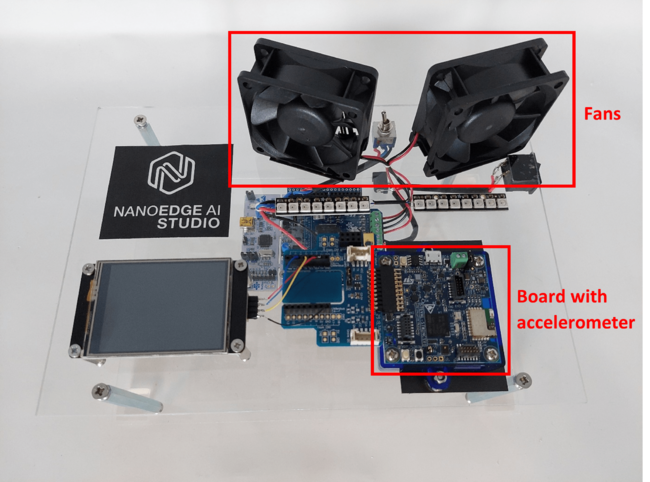
This is achieved using a 3-axis accelerometer. The sensor should be placed on the motor itself or as close to it as possible, to maximize the amplitude of the detected vibrations, and the accuracy of the analysis of the motor's behavior.
In this application, the signals used are temporal. Motors are modeled using 12V DC fans.
2.4.2. Initial thoughts
Even before starting data collection, it is necessary to analyze the use case, and think about the characteristics of the signal we are about to sample. Indeed, we want to make sure that we capture the essence of the physical phenomenon that takes place, in a way that it is mathematically meaningful for the Studio (that is, making sure the signal captured contains as much useful information as possible). This is particularly true with vibration monitoring, as the vibrations measured can originate from various sources and do not necessarily translate the motor's behavior directly. Hence the need for the user to be careful about the datalogging environment, and think about the conditions in which inferences are carried out.
Some important characteristics of the vibration produced can be noted:
- To consider only useful vibration patterns, accelerometer values must be logged when the motor is running. This is helpful to determine when to log signals.
- The vibration may be continuous on a short, medium or long-time scale. This characteristic must be considered to choose a proper buffer size (how long the signals should be, or how long the signal capture should take).
- Vibration frequencies of the different motor patterns must be considered to determine the target sampling frequency (output data rate) of the accelerometer. More precisely, the maximum frequency of the vibration impacts the minimum data rate allowing to reproduce the variations of the signal.
- The intensity of the vibration depends on the sensor's environment and motor regime. To record the maximum amplitude of the vibration and the most accurate patterns, the accelerometer should be placed as closed to the motor as possible. The maximum vibration amplitude must be considered to choose the accelerometer’s sensitivity.
2.4.3. Sampling frequency
While it may easy to determine the fundamental frequencies of sounds produced by a musical instrument (see 2.1.3), it is much more complex to guess which are the frequencies of the mechanical vibrations produced by a motor.
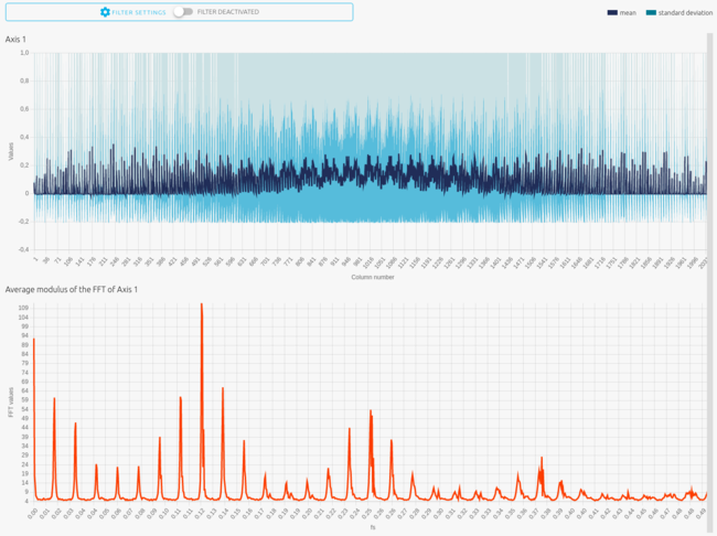
Therefore, to determine the best sampling frequency, we proceed by iterations. First, we set a medium frequency (among those available for our accelerometer): 833 Hz. We have chosen a signal length of 256 values. These settings allow to record patterns of 256/833 = 307 ms each. We can visualize the dataset in both temporal and frequential spaces in NanoEdgeAI Studio:
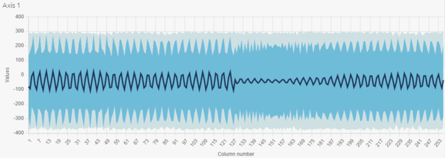
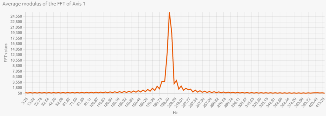
The recorded vibrations have one fundamental frequency. According to the FFT, this frequency is equal to 200 Hz.
The temporal view shows that we have logged numerous periods of vibrations in each signal (200 * 0,307 ~ 61 periods). So, the accuracy of the datalog is low (256 / 61 ~ 4 values per period).
Five or ten periods per signal are enough to have patterns representative of the motor behavior. The accuracy is the key point of an efficient datalog.
So we can begin the second iteration. We are going to increase the output data rate of the accelerometer to record a few periods per signal with a high accuracy.
The maximum output date rate we can set is 6667 Hz. This new setting allows to record patterns of 256/6667 = 38,4 ms each. Fundamental frequency of vibrations being equal to 200 Hz, we now record 200 * 0,0384 ~ 8 periods per signal.
Here are the temporal and frequential views of this new dataset:
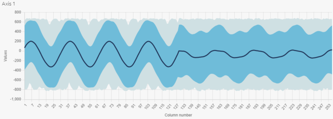
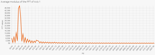
The vibrations logged here have a sinewave shape: the sampling frequency is sufficient to reproduce the entire signal. On the FFT graph, we note that the amplitude of the fundamental frequency is higher, and the harmonics are more visible. The signal is clearly more accurate. So a 6667 Hz sampling frequency is the most appropriate value in this example.
2.4.4. Buffer size
The buffer size is the number of samples composing our vibration signal. It should be a power of two for a proper data processing.
We have seen in the previous part that we record 8 periods of vibrations in a 256-sample buffer. We consider that signals containing 5 to 10 periods allow the most efficient processing by AI algorithms. So, our current length is optimal to have patterns representative of the motor behavior.
2.4.5. Sensitivity
The accelerometer used supports accelerations ranging from 2g up to 16g. Motors do not generate very ample vibrations, so a 2g sensitivity is enough in most cases. Sensitivity may be increased in case a saturation is observed in the temporal signals.
2.4.6. Signal capture
In order to capture every relevant vibration pattern produced by a running motor, two rules may be followed:
- Implement a trigger mechanism, to avoid logging when the motor is not powered. A simple solution is to define a threshold of vibration amplitude which is reached only when the motor is running.
- Set a random delay between logging 2 signals. This feature allows to begin datalogging at different signal phases, and therefore avoid recording the same periodic patterns continuously, which may in fact vary during the motors lifetime on the field.
The resulting 256-sample buffer is used as input signal in the Studio, and later on in the final device, as argument to the NanoEdge AI learning and inference functions.
Note: Each sample is composed of 3 values (accelerometer x-axis, y-axis and z-axis outputs), so each buffer contains 256*3 = 768 numerical values.
2.4.7. From signals to input files
Now that we managed to get a seemingly robust method to gather clean signals, we need to start logging some data, to constitute the datasets that are used as inputs in the Studio.
The goal is to be able to detect anomalies in the motor behavior. For this, we record 300 signal examples of vibrations when the motor is running normally, and 300 signal examples when the motor has an anomaly. We consider as an anomaly, a friction (applied to our prototype, a piece of paper rubbing fan blades) and an imbalance. For completeness, we record 150 signals for each anomaly. Therefore, we obtain the same amount of nominal and abnormal signals (300 each), which helps the NanoEdge AI search engine to find the most adapted anomaly detection library.
300 is an arbitrary number, but fits well within the guidelines: a bare minimum of 100 signal examples and a maximum of 10000 (there is usually no point in using more than a few hundreds to a thousand learning examples).
When recording abnormal signals, we make sure to introduce some amount of variety: for example, slightly different frictions on the blades. This increases the chances that the NanoEdge AI library obtained generalizes / performs well in different operating conditions.
Depending on the results obtained with the Studio, we adjust the number of signals used for input, if needed.
In summary:
- there are 3 input files in total, one nominal and one for each anomaly
- the nominal input file contains 300 lines, each abnormal input file contains 150 lines
- each line in each file represents a single, independent "signal example"
- there is no relation whatsoever between one line and the next (they could be shuffled), other than the fact that they testify to the same motor behavior
- each line is composed of 768 numerical values (3*256) (3 axes, buffer size of 256)
- each signal example represents a 38.4-millisecond temporal slice of the vibration pattern of the fans
2.4.8. Results
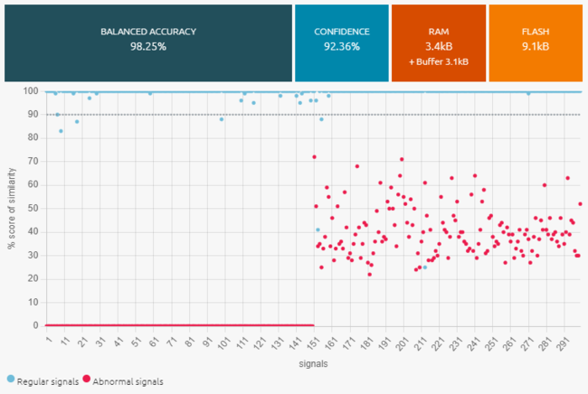
Here are the benchmark results obtained in the Studio with all our nominal and abnormal signals.
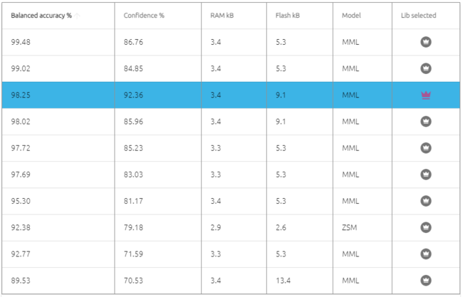
Here are some other candidate libraries that were found during benchmark, with their associated performances, memory footprint, and ML model info.
Observations:
- The best library found has very good performances.
- There is no need to adjust the datalogging settings.
- We could consider adjusting the size of the signal (taking 512 samples instead of 256) to increase the vibration patterns relevance.
- Before deploying the library, we could do additional testing, by collecting more signal examples, and running them through the NanoEdge AI Emulator, to check that our library indeed performs as expected.
- If collecting more signal examples is impossible, we could restart a new benchmark using only 60% of the data, and keep the remaining 40% exclusively for testing using the Emulator.
3. Resources