Datalogging guidelines for a successful NanoEdge AI project

This documents presents several use case studies where NanoEdge AI Studio has been used successfully to develop Anomaly Detection or Classification projects.

It aims at explaining the methodology and thought process behind the choice of crucial parameters during the initial datalogging process (that is, even before starting to use NanoEdge AI Studio) that can make or break a project.

For each use case, it will focus on the following aspects:

• what is a meaningful representation of the physical phenomenon being observed
• how to select the optimal sampling frequency for the datalogger
• how to select the optimal buffer size for the data sampled
• how to format the data logged properly for the Studio

1. Summary of important concepts

1.1. Definitions

Here are some clarifications regarding important terms that will be used in this document:

• "axis/axes": total number of variables outputted by a given sensor. Example: a 3-axis accelerometer outputs a 3-variable sample (x,y,z) corresponding to the instantaneous acceleration measured in 3 perpendicular directions.
• "sample": this refers to the instantaneous output of a sensor, and contains as many numerical values as the sensor has axes. For example, a 3-axis accelerometer outputs 3 numerical values per sample, while a current sensor (1-axis) outputs only 1 numerical value per sample.
• "signal", "signal example", or "learning example": used interchangeably, these refer to a collection of several samples, which has an associated temporal length (which depends on the sampling frequency used). The term "line" is also used to refer to a signal example, because in the input files for the Studio, each line represents an independent signal example.
• "buffer size", or "buffer length"; this is the number of samples per signal. It must be a power of 2. For example, a 3-axis signal with buffer length 256 is represented by 768 (256*3) numerical values.

1.2. Sampling frequency

The sampling frequency corresponds to the number of samples measured per second.

The speed at which the samples are taken must allow the signal to be accurately described, or "reconstructed"; the sampling frequency must be high enough to account for the rapid variations of the signal. The question of choosing the sampling frequency therefore naturally arises:

• If the sampling frequency is too low, the readings are too far apart; if the signal contains relevant features between two samples, they are lost.
• If the sampling frequency is too high, it may negatively impact the costs, in terms of processing power, transmission capacity, or storage space for example.

Important

To choose the sampling frequency, prior knowledge of the signal is useful in order to know its maximum frequency component. Indeed, to accurately reconstruct an output signal from an input signal, the sampling frequency must be at least twice as high as the maximum frequency that you wish to detect within the input signal. For more information, see Nyquist Frequency.

The issues related to the choice of sampling frequency and the number of samples are illustrated below:

• Case 1: the sampling frequency and the number of samples make it possible to reproduce the variations of the signal.

• Case 2: the sampling frequency is not sufficient to reproduce the variations of the signal.

• Case 3: the sampling frequency is sufficient but the number of samples is not sufficient to reproduce the entire signal (meaning that only part of the input signal is reproduced).

1.3. Buffer size

The buffer size corresponds to the total number of samples recorded per signal, per axis. Together, the sampling frequency and the buffer size put a constraint on the effective signal temporal length.

The buffer size must be a power of 2.

The buffer length must be chosen carefully, depending on the characteristics of the physical phenomenon sampled. For instance, the buffer may be chosen to be as short as a few periods in the case of a periodic signal (such as current, or stationary vibrations). In other cases, for instance when the signal is not purely periodic, the buffer size can be chosen to be as long as a complete operational cycle of the target machine to monitor (example: a robotic arm that moves from point A to point B, or a motor that ramps up from speed 1 to speed 2, and so on).

1.4. Data format

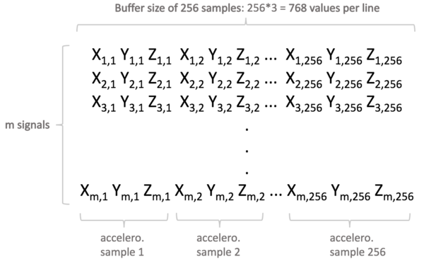
In the Studio, each signal is represented by an independent line, which format is completely constrained by the chosen buffer length and sampling frequency.

Important

In summary, there are three important parameters to consider: n: buffer size f: sampling frequency L: signal length They are linked together via: n = f * L. In other words, by choosing two (according to your use case), the third one is constrained.

Example:

Here is the input file format for a 3-axis sensor (in this example, an accelerometer), where the buffer size chosen is 256. Let's consider that the sampling frequency chosen is 1024 Hz. It means that each line (here, "m" lines in total) represents a temporal signal of 256/1024 = 250 milliseconds.

In summary, this input file contains "m" signal examples representing 250-millisecond slices of the vibration pattern the accelerometer is monitoring.

2. Use case studies

2.1. Vibration patterns on a ukulele

2.1.1. Context and objective

2.1.2. Implementation process

2.1.3. Results

2.2. Vibration patterns on an electric motor

2.2.1. Context and objective

2.2.2. Implementation process

2.2.3. Results

2.3. Current sensing on a 3-phase motor

2.3.1. Context and objective

2.3.2. Implementation process

2.3.3. Results

2.4. Gesture recognition using a Time-of-Flight sensor

2.4.1. Context and objective

2.4.2. Implementation process

2.4.3. Results

3. Resources