This documents presents several use case studies where NanoEdge AI Studio has been used successfully to create smart devices with machine learning features using a NanoEdge AI library.
It aims at explaining the methodology and thought process behind the choice of crucial parameters during the initial datalogging phase (that is, even before starting to use NanoEdge AI Studio) that can make or break a project.
For each use case, it will focus on the following aspects:
- what is a meaningful representation of the physical phenomenon being observed
- how to select the optimal sampling frequency for the datalogger
- how to select the optimal buffer size for the data sampled
- how to format the data logged properly for the Studio
1. Summary of important concepts
1.1. Definitions
Here are some clarifications regarding important terms that will be used in this document:
- "axis/axes": total number of variables outputted by a given sensor. Example: a 3-axis accelerometer outputs a 3-variable sample (x,y,z) corresponding to the instantaneous acceleration measured in 3 perpendicular directions.
- "sample": this refers to the instantaneous output of a sensor, and contains as many numerical values as the sensor has axes. For example, a 3-axis accelerometer outputs 3 numerical values per sample, while a current sensor (1-axis) outputs only 1 numerical value per sample.
- "signal", "signal example", or "learning example": used interchangeably, these refer to a collection of numerical values that are used as input in the NanoEdge AI functions, either for learning of for inference. The term "line" is also used to refer to a signal example, because in the input files for the Studio, each line represents an independent signal example.
- "buffer size", or "buffer length"; this is the number of samples per signal. It must be a power of 2. For example, a 3-axis signal with buffer length 256 is represented by 768 (256*3) numerical values.
1.2. Sampling frequency
The sampling frequency, sometimes referred to as (output) data rate, corresponds to the number of samples measured per second.
The speed at which the samples are taken must allow the signal to be accurately described, or "reconstructed"; the sampling frequency must be high enough to account for the rapid variations of the signal. The question of choosing the sampling frequency therefore naturally arises:
- If the sampling frequency is too low, the readings are too far apart; if the signal contains relevant features between two samples, they are lost.
- If the sampling frequency is too high, it may negatively impact the costs, in terms of processing power, transmission capacity, or storage space for example.
The issues related to the choice of sampling frequency and the number of samples are illustrated below:
- Case 1: the sampling frequency and the number of samples make it possible to reproduce the variations of the signal.

- Case 2: the sampling frequency is not sufficient to reproduce the variations of the signal.

- Case 3: the sampling frequency is sufficient but the number of samples is not sufficient to reproduce the entire signal (meaning that only part of the input signal is reproduced).

1.3. Buffer size
The buffer size corresponds to the total number of samples recorded per signal, per axis. Together, the sampling frequency and the buffer size put a constraint on the effective signal temporal length.
The buffer size must be a power of 2.
The buffer length must be chosen carefully, depending on the characteristics of the physical phenomenon sampled. For instance, the buffer may be chosen to be as short as a few periods in the case of a periodic signal (such as current, or stationary vibrations). In other cases, for instance when the signal is not purely periodic, the buffer size can be chosen to be as long as a complete operational cycle of the target machine to monitor (example: a robotic arm that moves from point A to point B, or a motor that ramps up from speed 1 to speed 2, and so on).
In some cases, where the signal considered is not temporal (example: time-of-flight sensor), the buffer size is simply constrained by the size and resolution of the sensor's output (for instance, a buffer size of 64 for a 8x8 time-of-flight array).
1.4. Data format
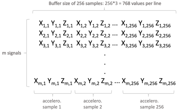
In the Studio, each signal is represented by an independent line, which format is completely constrained by the chosen buffer length and sampling frequency.
Example:
Here is the input file format for a 3-axis sensor (in this example, an accelerometer), where the buffer size chosen is 256. Let's consider that the sampling frequency chosen is 1024 Hz. It means that each line (here, "m" lines in total) represents a temporal signal of 256/1024 = 250 milliseconds.
In summary, this input file contains "m" signal examples representing 250-millisecond slices of the vibration pattern the accelerometer is monitoring.
2. Use case studies
2.1. Vibration patterns on a ukulele
2.1.1. Context and objective
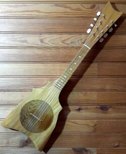
In this project, the goal is to capture the vibrations produced when the ukulele is strummed, in order to be able to classify them, based on which individual musical note, or which chord (superposition of up to 4 notes), is played.
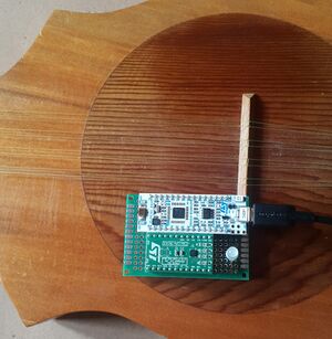
A 3-axis accelerometer is placed directly on the ukulele, or in the sounding box, wherever the vibrations are expected to be most intense.
2.1.2. Initial thoughts
Even before starting data collection, it is necessary to analyze the use case, and think about the characteristics of the signal we are about to sample. Indeed, we want to make sure that we capture the essence of the physical phenomenon that takes place, in a way that will be mathematically meaningful for the Studio (that is, making sure the signal captured contains as much useful information as possible).
When strumming the ukulele, some important characteristics of the vibration produced can be noted:
- The action of strumming is sudden, therefore the signal created is a burst of vibration, and dies off after a couple of seconds. The vibration may be continuous on a short time scale, but it does not last long, and is not periodic on a medium or long time scale. This will be helpful to determine when to start signal acquisition.
- The previous observation will also be useful to choose a proper buffer size (how long the signals should be, or how long the signal capture should take).
- The frequencies involved in the vibration produced are clearly defined, and can be identified through the pitch of the sound produced. This will be helpful to determine the target sampling frequency (output data rate) of the accelerometer.
- The intensity of the vibrations are somewhat low, so we'll have to be careful about where to place the accelerometer on the ukulele's body, and how to choose the accelerometer's sensitivity.
2.1.3. Sampling frequency
When strumming the ukulele, all the strings vibrate at the same time, which makes the ukulele itself vibrate. This produces the sound that we hear, so we can assume that the sound frequencies, and the ukulele vibration frequencies, are closely related.
Each chord contains a superposition of 4 musical notes, or pitches. This means we have 4 fundamental frequencies (or base notes) plus all the harmonics (which give the instrument its particular sound). These notes are quite high-pitched, compared to a piano for example. For reference, we humans can usually hear frequencies between 20 and 20000 Hz, and that the note A (or la) usually has a fundamental frequency of 440 Hz. So we can estimate that the chords played on the ukulele contain notes between 1000 and 10000 Hertz maximum.
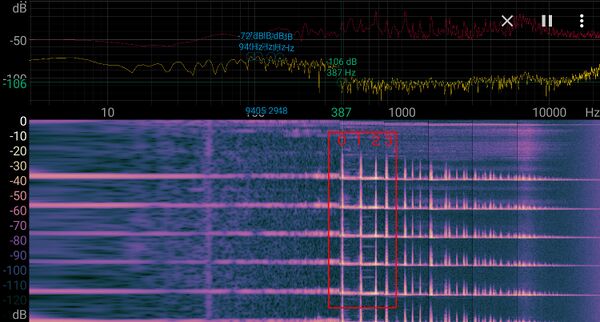
To be more precise, we can use a simple frequency analyzer. In this example, we are using Spectroid, a free Android app.
Here is the spectrogram obtained when playing the C major chord (or do) several times.
Here's the spectrogram on a F major chord (fa).
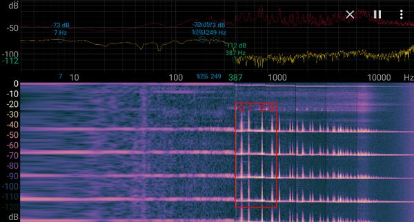
In both cases, the fundamental frequency (0) and the 3 first harmonics (1, 2, 3) are between around 380 and 1000 Hz. There are many more harmonics up to 10 kHz, but they rapidly decrease in intensity, so we can assume for the moment that 1000 Hz is the maximum frequency to sample.
To do so, we need to set the sampling frequency to at least double that frequency; 2000 Hz minimum.
In this example, the accelerometer used only supports a discrete range of sampling frequencies, among which: 1666 Hz, 3333 Hz and 6666 Hz.
We will start testing with a sampling frequency of 3333 Hz. We will adapt later, depending on the results we get from the Studio, for instance by doubling the frequency to 6666 Hz for more precision.
2.1.4. Buffer size
The buffer size is the number of samples composing our vibration signal.
When strumming the ukulele, the sound produced lasts for one second or so. The vibration on the ukulele body quickly dies off, so we can assume that capturing a signal of maximum 0.5 seconds will be enough. We will adapt later, depending on the results we get from the Studio.
With a target length of approximately 0.5 seconds, and a sampling frequency of 3333 Hz, we get a target buffer size of 3333*0.5 = 1666.
The chosen buffer size should be **a power of two**, so we'll go with 1024 instead of 1665. We could have picked 2048, but 1024 samples is enough for a first test. We can always increase it later if required.
As a result, the sampling frequency of 3333 Hz with the buffer size of 1024 (samples per signal per axis) make a recorded signal length of 1024/3333 = 0.3 seconds approximately.
So each signal example that is used for data logging, or passed to a NanoEdge AI function for learning or inference, will represent a 300-millisecond slice of vibration pattern. During these 300 ms, all 1024 samples are recorded continuously. But since all signal examples are independent from one another, whatever happens between two consecutive signals does not matter (signal examples don't have to be recorded at precise time intervals, or continuously).
iii. Accelerometer sensitivity
The LSM6DSL supports accelerations ranging from 2g up to 16g. For gentle ukulele strumming, 2g or 4g should be enough (we can always adjust it later).
We choose a sensitivity of 4g. This is reflected in the following line of code.
.. code-block:: c
lsm6dsl->set_x_fs(4.0f);
.. _trigger:
iv. Signal capture
In order to create our signals, we can imagine continually recording accelerometer data. However, we chose an actual signal length of 0.3 seconds. So if we started strumming the ukulele randomly, with continuous signal acquisition, we would end up with messy signals. Namely, on our 0.3 second window (1024 samples) we would have no guarantee that the relevant signals are captured. Also, a lot of "silence" would be recorded, between strums.
Instead, we implement a **trigger mechanism**; everytime the intensity of the ukulele vibrations are higher than a **threshold**, we trigger the capture of a single signal (1024 samples). To do so, we continually monitor vibration patterns, and record them into two consecutive mini-buffers. The average x, y, z accelerations of these buffers are then compared, and if the vibration intensity of the 2nd buffer if higher that that of the 1st (times a threshold), the trigger is activated, and a signal is recorded. See the code in *main.cpp* in the function ``strum_trigger`` for more details.
.. important::
Depending on your instrument you may need to adjust the trigger behavior by changing the following parameters in ``main.cpp``:
.. code-block:: c
        #define MINI      5        /* The size of a mini-buffer */
        #define THRESH    1.4      /* The threshold (multiplier) used for trigger (40%) */
        #define NOISE     0.15     /* The minimum vibration intensity to consider */
     | Go to *Studio Step 2: Regular signals* > *Choose signals* > *From serial (USB)*.
     | Make sure you attached the data logger to your instrument (see :ref:`this section <attach>`).
     | Click the **Record button**, and check that strumming your instrument triggers signal recording (repeat a few times).
If you find that signals fail to be triggered, try one (or both) of the following:
        * decrease the ``THRESH`` multiplier by increments of 0.05 (e.g. *1.35* and so on);
        * decrease the ``NOISE`` level by increments of 0.05 (lowering it *to 0* if required).
If you find that signals are triggered too often, try one (or both) of the following:
        * increase ``THRESH`` by increments of 0.05 (e.g. *1.35*, *1.3* and so on);
        * increase ``NOISE`` by increments of 0.05 (e.g. *0.2*, *0.25* and so on).