1. What is NanoEdge AI Library?
NanoEdge™ AI Library is an Artificial Intelligence (AI) static library originally developed by Cartesiam, for embedded C software running on Arm® Cortex® microcontrollers (MCUs). It comes in the form of a precompiled .a file that provides building blocks to implement smart features into any C code.
When embedded on microcontrollers, the NanoEdge AI Library gives them the ability to "understand" sensor patterns automatically, by themselves, without the need for the user to have additional skills in Mathematics, Machine Learning, or data science.
Each NanoEdge AI static library contains an AI model designed to bring Machine Learning capabilities to any C code, in the form of easily implementable functions, e.g., for learning signal patterns, detecting anomalies, classifying signals, or extrapolating data.
There are 4 different types of NanoEdge AI Libraries, corresponding to the 4 types of projects that can be created in NanoEdge AI Studio:
- Anomaly Detection (AD) libraries are used to detect abnormal behaviors on a machine, after an initial in-situ training phase, using a dynamic model that learns patterns incrementally.
- n-class Classification (nCC) libraries are used to distinguish and recognize different types of behaviors, anomalous or not, and classify them into pre-established categories, using a static model.
- 1-class Classification (1CC) libraries are used to detect abnormal behaviors on a machine, using a static model, without providing any context about the possible anomalies to be expected.
- Extrapolation (EX) libraries are used to estimate an unknown target value using other know parameters, using a static (regression) model.
Here are the most important features of the NanoEdge AI Libraries:
- ultra optimized to run on MCUs (any Arm® Cortex®-M)
- ultra memory efficient (1-20 Kbytes of RAM/Flash memory)
- ultra fast (1-20 ms inference on Cortex®-M4 at 80 MHz)
- inherently independent from the cloud
- run directly within the microcontroller
- can be integrated into existing code / hardware
- consume very little energy
- preserve the stack (static allocation only)
- transmit or save no data
- require no Machine Learning expertise to be deployed
All NanoEdge AI Libraries are created by using NanoEdge AI Studio.
2. Purpose of NanoEdge AI Studio
2.1. What the Studio can do
NanoEdge AI Libraries contains a range of Machine Learning models, and each of these models can be optimized by tuning a wide range of hyperparameters. This results in a very large number of potential combinations, each one being tailored for a specific use-case (one static libraries for each combination). Therefore, a tool is needed to find the best possible library for each project.
NanoEdge AI Studio (NanoEdgeAIStudio), also referred to as the Studio,
- is a search engine for AI Libraries
- is built for embedded developers
- abstracts away all aspects of Machine Learning and data science
- enables the quick and easy development of Machine Learning capabilities into any C code
- uses minimal amounts of input data compared to traditional Machine Learning approaches
Its purpose is to find the best possible NanoEdge AI static library for a given hardware application, where the only requirements in terms of user knowledge are embedded development (software/hardware), C coding, and basic signal sampling notions.
NanoEdge AI Studio takes as input project parameters (such as MCU type, RAM and sensor type) and some signal examples, and outputs the most relevant NanoEdge AI Library. This library can either be untrained (it will only start learning after it is embedded in the microcontroller) or pre-trained in the Studio. In all cases, the NanoEdge AI Library will be able to infer (detect, classify, extrapolate...) directly from the target microcontroller.
The resulting NanoEdge AI Library is a combination of 3 elementary software bricks:
- signal pre-processing algorithm (e.g. FFT, PCA, normalization, reframing...),
- Machine Learning model (e.g. kNN, SVM, neural networks, Cartesiam-proprietary ML algorithms...),
- optimal hyperparametrization for the ML model.
Each NanoEdge AI static library is the result of the benchmark of virtually all possible AI libraries (combinations of signal treatment, ML model and tuned hyperparameters), tested against the minimal data given by the user. It therefore contains the best possible model, for a given use case, given the signal examples provided as input.
Using NanoEdge AI Studio is an iterative process by design: users can import signals, run a benchmark, find a library, and start testing it in under an hour.
Then, depending on the results obtained, changes are made to the input data (quality and/or quantity of signals), and the process restarted, to obtain a better iteration of the NanoEdge AI Library.
2.2. What the Studio cannot do
In a nutshell, NanoEdge AI Studio takes user data as input (in the form of sensor signal examples), and produces a static library (.a) file as output. This is a straightforward and relatively quick iterative procedure.
However, the Studio does not provide any input data. The user needs to have qualified data (of sufficient quality and quantity) in order to obtain satisfactory results from the Studio. This data can either be raw sensor signals, or pre-treated signals, and need to be formatted properly (see below). For example, for anomaly detection on a machine, the user needs to collect signal examples representing "normal" behaviors on this machine, as well as a few examples of possible "anomalies". This data collection process is crucial, and can be tedious, as some expertise is needed to design the correct signal acquisition and sampling methodology, which can vary dramatically from one project to the other.
Additionally, NanoEdge AI Studio does not provide any ready-to-use C code to implement in your final project. This code, which includes some of the NanoEdge AI Library smart functions (e.g., init, learn, detect, classification, extrapolation), needs to be written and compiled by the user. The user is free to call these functions as needed, and implement all the smart features imaginable.
In summary, the static (.a) library file, outputted by the Studio from user-generated input data, must be linked to some C code written by the user, and compiled/flashed by the user on the target microcontroller.
3. Getting started
NanoEdge AI Studio can be used to generate ML libraries for different project types, using data coming from one or more sensors, possibly of different types. It is therefore crucial to understand which project type to create for a given use case, and which sensor type will be most relevant to use.
3.1. Defining important concepts
Some vocabulary used in this documentation may be interpreted in different ways depending on the context. Here are some clarifications:
- "axis/axes" and "variable(s)": here these two terms will be used interchangeably.
- "sample": this refers to the instantaneous output of a sensor, and contains as many numerical values as the sensor has axes (or variables). For example, a 3-axis accelerometer outputs 3 numerical values per sample, while a current sensor (1-axis) outputs only 1 numerical value per sample.
- "signal", "signal example", or "learning example": used interchangeably, these refer to a collection of several samples, which has an associated temporal length (which depends on the sampling frequency used). The term "line" will also be used to refer to a signal example, because in the input files for the Studio, each line represents an independent signal example (exception: Multi-sensor, see below).
- "buffer size", or "buffer length"; this is the number of samples per signal. It should be a power of 2. For example, a 3-axis signal with buffer length 256 will be represented by 768 (256*3) numerical values.
3.2. Types of projects in NanoEdge AI Studio
The 4 different types of projects that can be created using the Studio, along with their characteristics, outputs, and possible use cases, are outlined below:
Anomaly Detection (AD):
- Use case: detecting anomalies in data using a dynamic model.
- User input: signal examples representing both nominal states and abnormal states (used for library selection only).
- Studio output: untrained anomaly detection library that will learn incrementally, directly on the target microcontroller.
1-class Classification (1CC):
- Use case: detecting anomalies in data using a static model.
- User input: signal examples representing normal states only (used for both library selection and model training).
- Studio output: pre-trained outlier detection library that will infer directly on the target microcontroller.
n-class Classification (nCC):
- Use case: distinguishing among n different states using a static model.
- User input: signal examples representing all the different states (classes) to be expected (used for both library selection and model training).
- Studio output: pre-trained classification library that will infer directly on the target microcontroller.
Extrapolation (EX):
- Use case: estimating an unknown target value using other know parameters, using a static model.
- User input: signal examples associating the know parameters, to their target values (used for both library selection and model training).
- Studio output: pre-trained regression library that will infer directly on the target microcontroller.
3.3. Types of sensors in NanoEdge AI Studio
NanoEdge AI Studio and its output NanoEdge AI Libraries are compatible with any sensor type; they are sensor-agnostic. For example, users may use data coming from an accelerometer, a magnetometer, a microphone, a gas sensor, a time-of-flight sensor, a microphone, or a combination of any of these (list non exhaustive).
The Studio is designed to be able to work with raw sensor data, that hasn't necessarily been pre-processed. However, in cases where users already have some knowledge and expertise about their signals, pre-processed signals can be imported instead.
Depending on the user's use case, the Studio needs to understand which data format to expect in the imported input files. There are 2 main categories of sensors selectable in the Studio:
- Generic (n axes) sensor, which is a generalization of some other sensor types, e.g., accelerometer 3 axes, magnetometer 1 axis, microphone (1 axis), current (1 axis), and so on. This sensor covers most typical use cases, and will be selected most of the time.
- Multi-sensor (n variables), referred to as "Multi-sensor", which is specific to anomaly detection projects, and designed for niche use cases, for which the expected format is entirely different.
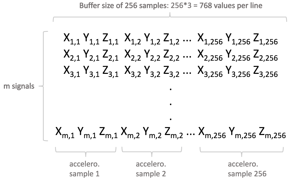
The Generic n-axis sensor (and all others except "Multi-sensor") expects a buffer of data as input, in other words, a signal example represented by a succession of instantaneous sensor samples. As a result, this "signal example" will have an associated temporal length, which depends on the sampling frequency (output data rate of the sensor) and on the number of instantaneous samples composing the signal example (referred to as buffer size, or buffer length).
The Multi-sensor sensor, on the other hand, expects instantaneous samples of data. In other words, it uses a single sensor sample as input, as opposed to a temporal signal example composed of many samples.
In the remainder of this documentation, except when explicitly stated otherwise, the "Generic" sensor approach (using signal examples / buffers as input, rather that single samples) will be used by default.
3.4. Designing a relevant sampling methodology
Compared to traditional machine learning approaches, which may require hundreds of thousands of signal examples to build a model, NanoEdge AI Studio requires minimal input datasets (as little as 50-100 signal examples, depending on the use case).
However, this data needs to be qualified, which means that it must contain relevant information about the physical phenomena to be monitored. For this reason, it is absolutely crucial to design the proper sampling methodology, in order to make sure that all the desired characteristics from the physical phenomena to be sampled are correctly extracted and translated into meaningful data.
To prepare input data for the Studio, the user must choose the most adequate sampling frequency.
The sampling frequency corresponds to the number of samples measured per second. For some sensors, the sampling frequency can be directly set by the user (e.g. digital sensors), but in other cases (e.g. analog sensors), a timer needs to be set up for constant time intervals between each sample.
The speed at which the samples are taken must allow the signal to be accurately described, or "reconstructed"; the sampling frequency must be high enough to account for the rapid variations of the signal. The question of choosing the sampling frequency therefore naturally arises:
- If the sampling frequency is too low, the readings are too far apart; if the signal contains relevant features between two samples, they are lost.
- If the sampling frequency is too high, it may negatively impact the costs, in terms of processing power, transmission capacity, or storage space for example.
The issues related to the choice of sampling frequency and the number of samples are illustrated below:
- Case 1: the sampling frequency and the number of samples make it possible to reproduce the variations of the signal.

- Case 2: the sampling frequency is not sufficient to reproduce the variations of the signal.

- Case 3: the sampling frequency is sufficient but the number of samples is not sufficient to reproduce the entire signal (meaning that only part of the input signal is reproduced).

The buffer size corresponds to the total number of samples recorded per signal, per axis. Together, the sampling frequency and the buffer size put a constraint on the effective signal temporal length.
Here are general recommendations. Make sure that:
- the sampling frequency is high enough to catch all desired signal features. To sample a 1000 Hz phenomenon, you must at least double the frequency (in this case, sample at 2000 Hz at least).
- your signal is long (or short) enough to be coherent with the phenomenon to be sampled. For example, if you want your signals to be 0.25 seconds long (
L), you must haven / f = 0.25. For example, choose a buffer size of 256 with a frequency of 1024 Hz, or a buffer of 1024 with a frequency of 4096 Hz, and so on.
3.5. Preparing signal files
During the library selection process, NanoEdge AI Studio uses user data (input files containing signal examples) to test and benchmark many signal preprocessing algorithms, Machine Learning models and parameters. The way these input files are structured, formatted, and the way the signal were recorded is therefore very important.
Here are general considerations for input file format, which apply to all cases. The Studio expects:
- .txt / .csv files
- numerical values only (not counting separators), and no headers
- uniform separators throughout the whole file: either
single space,tab,,or;. - decimal values formatted using a period (
.) and not commas (,). - more than 1 sample per line (exception: Multi-sensor)
- fewer than 16384 (214) values per line
- the same number of numerical values on each line
- a bare minimum of 20 lines per sensor axis (e.g. for a 3-axis accelerometer: 60 lines is a bare minimum)
- fewer than ~100000 lines in total (generally, 50-1000 are more than enough)
- file size lower than ~1 Gb
Then, there are some specific formatting rules, mainly depending on the type of project created in the Studio:
- Anomaly detection, 1-class classification, and n-class classification projects all follow the same general rules.
- Extrapolation projects has a particularity, because it needs to incorporate the target values from which to extrapolate.
- Multi-sensor is a big exception, and applies only to niche cases in anomaly detection projects.
3.5.1. General rules
The following applies to anomaly detection (exception: Multi-sensor), 1-class classification, and n-class classification projects.
In NanoEdge AI Studio, lines are taken into account independently, iteratively, so they must represent a meaningful snapshot in time of the signal to be processed. It it therefore crucial to set a coherent sampling frequency and a proper buffer size.
The Studio expects:
- each line to represent a single, independent signal example, made of many samples
- the buffer size of this signal to be a power of two, and to stay constant throughout the project
- the sampling frequency of this signal to stay constant throughout the project
- all signal examples corresponding to a given "class" to be combined in the same input file (for anomaly detection, it generally means that all "nominal" regimes should be concatenated into a single "nominal" input file, and all "abnormal regimes" into a single "anomalies" input file.
Example:
I am using a 3-axis accelerometer. I want to monitor a piece of equipment that vibrates. I will collect a total of 100 learning examples to represent the vibration behavior of my equipment. I estimate the highest-frequency component of this vibration to be below 500 Hz, therefore I choose a sampling frequency of 1000 Hz for my sensor. I decide that my learning examples for this vibration should represent about 1/4 of a second (250 ms). To achieve this, I choose a buffer size of 256 samples. This means my 256 samples will represent a signal of 1000/256 = 256 ms.
Therefore, in my input file, each signal will be composed of 256 3-value samples. This means each of the 100 lines in my input file will be composed of 768 numerical values (256*3).
3.5.2. Variant: Extrapolation projects
The following applies to extrapolation projects only.
The mathematical models used in NanoEdge AI Extrapolation libraries are regression models (not necessarily linear). Therefore, all general information and rules governing regression apply here.
NanoEdge AI Studio uses input files provided in Extrapolation projects both to find the best possible NanoEdge AI Extrapolation library, and also to train it. It means that the learning examples (lines) provided in the input files should not only contain the signal buffer itself, but also the target values associated to this signal buffer.
The point is to learn a model that will correlate each signal buffer to a target value, so that after training, when it is embedded into the microcontroller, the extrapolation library is able to read a signal buffer, and infer the missing (unknown) target value.
Input file format provided to the Studio for extrapolation only slightly differ from the general guidelines presented in the previous section. The difference is that the signal buffer (each line) should be preceded by a single numerical value, representing the target to evaluate, as shown here:
These target values are provided in the Studio for library selection / training, but omitted during testing.
Therefore, during testing (e.g. using the NanoEdge AI Emulator), the input file format is exactly the same as the one described in the previous section, titled "General rules".
Example:
I'm trying to evaluate / predict / extrapolate my running speed (which is my target value) from raw 3-axis accelerometer data.
- I choose a sampling frequency of 500 Hz on my accelerometer (which I believe will be sufficient to capture all vibratory characteristics or my "running signature"), and a buffer size of 1024 (because at 500 Hz it will represent a temporal signal segment of approximately 2 seconds, which I estimate will contain sufficient information to extrapolate a speed).
- I also need a way to measure my running speed (target value), in order to train the model later on. For instance, I can use a (GPS) speedometer, or simply run a known distance and record my time.
- Then, I can start collecting data.
I will walk / run several times while carrying my speedometer and accelerometer, to collect both accelerometer buffers and the associated speeds.
For instance, I will walk / run 6 times, at 6 noticeably different speeds, each time for 1 minute at constant speed. Therefore for each run, I will get one known speed value, and many (approximately 30) two-second accelerometer buffers composed of 1024*3 = 3072 values each. - Finally, I compile this data in a single file that I will use as input in the Studio.
- This file contains approximately 180 lines (6 runs with 30 buffers each), each representing an individual training example.
- Each line is composed of 3073 numerical values: 1 speed value followed by 1024*3 accelerometer values, all separated (for example) by commas.
- The first 30 lines all start with the same speed value, but have different associated accelerometer buffers (1st run). The 30 next lines all start with another speed value, and have their associated accelerometer buffers (2nd run), and so on.
- After my model is trained, I am able to evaluate my running speed, just by providing the best NanoEdge AI library found by the Studio, with some accelerometer buffers of size 1024 sampled at 500 Hz (of course, without providing the speed value). The data provided for inference (or testing) therefore contains 3072 values only (no speed), since speed is what I'm trying to estimate.
3.5.3. Exception: Multi-sensor
In anomaly detection projects (only), the Multi-sensor sensor is used to monitor machine "states" that typically evolve slowly in time. These states may be represented by variables coming from distinct sensor sources, and/or result from the aggregation of signal buffers into artificial, higher level features.
Here, the input format is different:
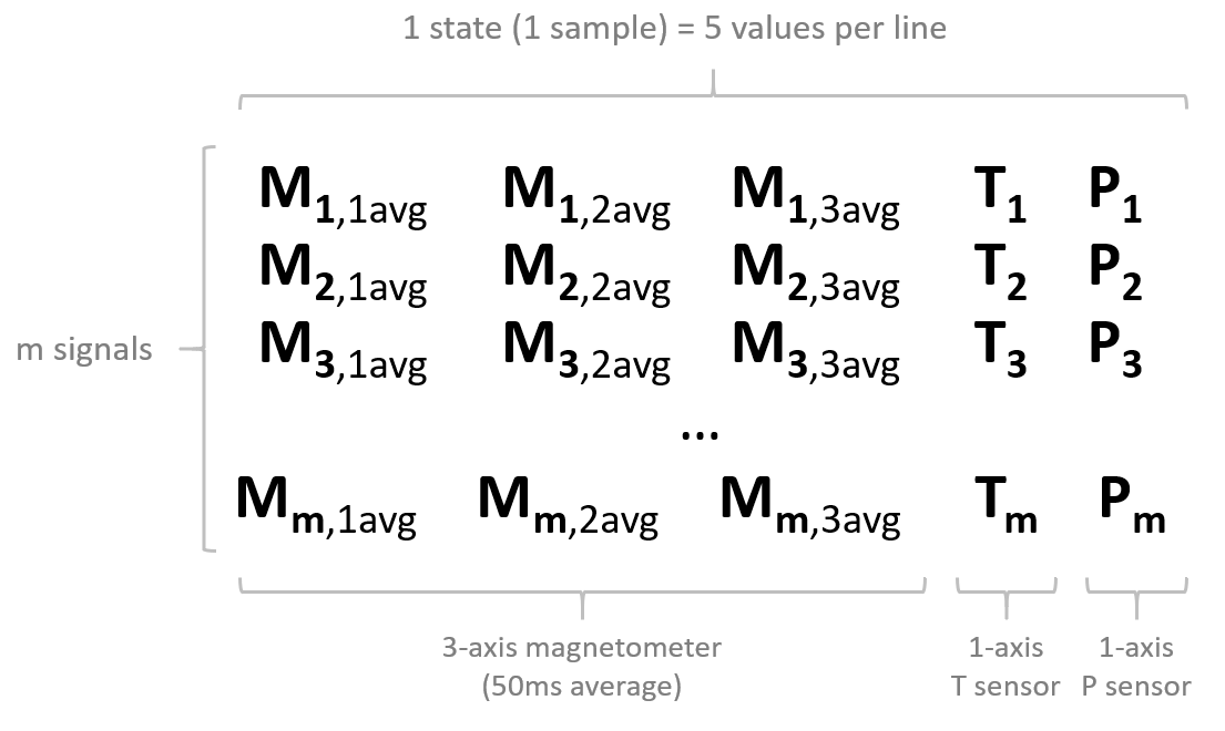
- Each line represents a single sample (possibly multi-variable) instead of a full signal.
- The number of values per line (equal to the number of variables per sample) does not have to be a power of two.
- The lines are not independent, so the ordering does matter (lines should not be shuffled).
- Typically, there are many more lines in the input file compared to the "normal" case (not "Multi-sensor"), since we now have only one sample per line, instead of many samples per line.
Example:
I want to monitor the state of a machine, represented by a combination of sensors; 3-axis magnetometer, a temperature sensor (1 axis), and a pressure sensor (1-axis). Temperature and pressure, if they vary slowly, can be read directly, but magnetometer data needs to be summarized using (for example) average values across a 50 millisecond window along all 3 axes (we do not use instantaneous values). This would result in 3 extracted magnetic features, followed by temperature, followed by pressure, to represent a 5-variable state.
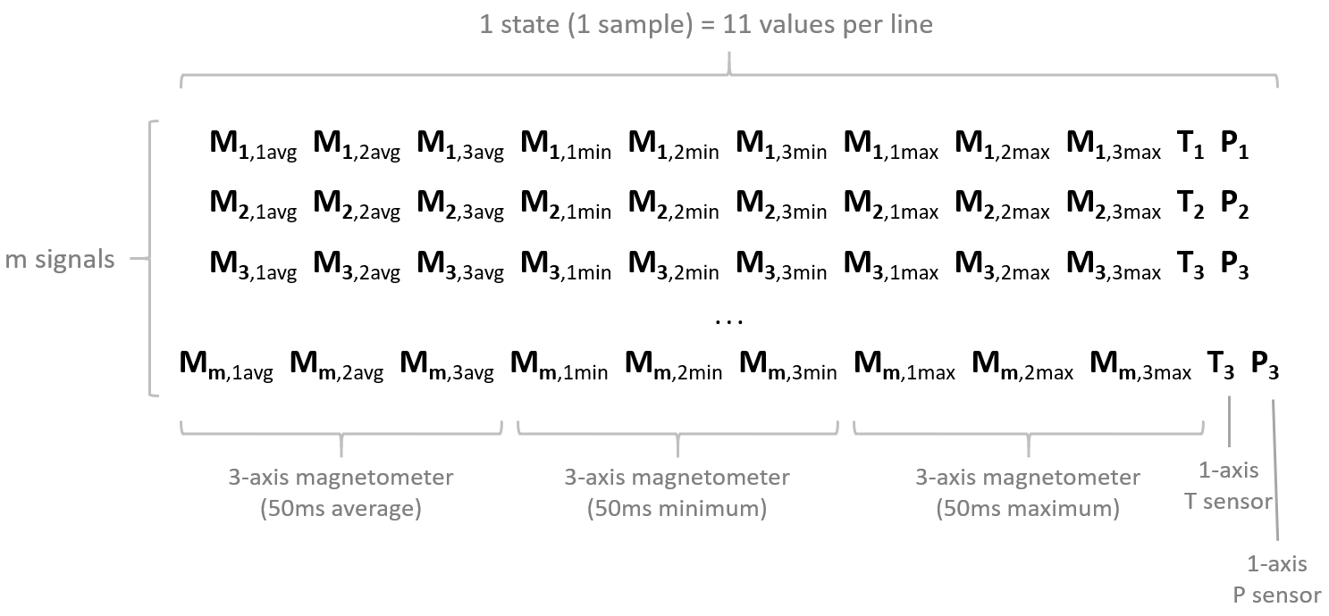
We could also imagine building a more complex state from our 50 millisecond magnetometer buffer, including not only average magnetometer values, but also minima and maxima, for all 3 axes. This would result in 3*3 = 9 extracted magnetometer values (3 each for average, minimum, maximum), followed by temperature and pressure, to represent a 11-variable state.
4. Using NanoEdge AI Studio
4.1. Running NanoEdge AI Studio for the first time
When running NanoEdge AI Studio for the first time, you are prompted for:
- Your proxy settings: if you are using a proxy, use the settings below, otherwise, click NO.
- Here are the IP addresses that need to be authorized:
Licensing API: Cartesiam API for library compilation: 54.147.158.222 52.178.13.227 54.147.163.93 - 54.144.124.187 - 54.144.46.201 - or via URL: https://api.cryptlex.com:443 or via URL: https://api.nanoedgeaistudio.net (alternatively, https://api.cartesiam.net)
- The port you want to use.
- It can be changed to any port available on your machine (port 5000 by default).
- Your license key.
- If you do not know your license key, log in to the Cryptex licensing platform to retrieve it.
- If you have lost your login credentials, reset your password using the email address used to download NanoEdge AI Studio.
- If you do not know your license key, log in to the Cryptex licensing platform to retrieve it.
4.2. Studio's home screen
The Studio main (home) screen comprises 4 main elements:
- The project creation bar (top)
- The existing projects window (left side)
- The "inspiration" window (right side)
- The toolbar (left extremity)
The project creation bar [1] is used to create a new project (anomaly detection, 1-class classification, n-class classification, or extrapolation), or to create a data logger (specific to STEVAL-STWINKT1B) in order to quickly start gathering data using a wide range of sensors, and easily import it into the Studio.
The existing projects window [2] is used to load, import/export, or search existing NanoEdge AI projects.
The inspiration window [3] provides links to the Use Case Explorer data portal, where datasets corresponding to a wide range of interesting use cases are publicly available for download. This data portal also contains summaries of the performances obtained with NanoEdge AI Studio using these datasets.
The toolbar [4] provides quick access to:
- the Studio settings (port, workspace folder path, license information, and proxy settings)
- the NanoEdge AI documentation
- NanoEdge AI's license agreement
- CLI (command line interface client) download
- Studio log files (for troubleshooting)
- the Studio workspace folder
4.3. Creating a new project
On the main screen, select your desired project type on the project creation bar, and click CREATE NEW PROJECT.
Each project is divided into 5 successive steps:
- Global settings, to set the general project parameters
- Signals, to import signal examples that will be used for library selection.
Note: this step is divided in 2 substeps in anomaly detection projects (Regular signals / Abnormal signals) - Optimize & benchmark, where the best NanoEdge AI Library is automatically selected and optimized
- Emulator, to test the candidate libraries before embedding them into the microcontroller
- Deploy, to compile and download the best library and its associated header files, ready to be linked to any C code.
4.3.1. Global settings
The first step in any project is Global settings.
Here, the following parameters parameters will be set:
- Project name
- Description (optional)
- Max RAM: this is the maximum amount of RAM memory to be allocated to the AI library. It doesn't take into consideration the space taken by the sensor buffers.
- Limit Flash / No Flash limit: this is the maximum amount of Flash memory to be allocated to the AI library.
- Sensor type: the type of sensor used to gather data in the project, and the number of axes / variables when using a "Generic" sensor or "Multi-sensor".
- Target: this is the type of board / microcontroller on which the final NanoEdge AI Library will be deployed.
The trial version of NanoEdge AI Studio is limited to the following boards:- STEVAL-STWINKT1B
- Disco-B-U585I-IOT02A
- Disco-F413ZH
- Disco-F746NG / F769NI
- Disco-L4R9I / L4S5I
- Disco-L562E
- Nucleo-F401RE / F411RE
- Nucleo-G071RB
- Nucleo-G474RE
- Nucleo-H743ZI2
- Nucleo-L432KC / L433RC-P / L476RG
- Nucleo-WB55RG / WL55JC
4.3.2. Signals
4.3.2.1. How to import signals
The input files, containing all the signal examples to be used by the Studio to select the best possible AI library, may be imported from 3 sources:
- From a file (in .txt / .csv format)
- From the serial port (USB) of a live datalogger
- From the SD card of a datalogger (in .dat format), obtained via the Datalogger feature of the Studio (see this section).
1. From file:
- Click SELECT FILES, and select the input file to import.
- Rename the input file if needed.
- Repeat the operation to import more files.
- Click CONTINUE.
2. From serial port:
- Select the COM Port where your datalogger is connected, and select the correct Baudrate.
- If needed, tick the checkbox enter a maximum number of lines to be imported.
- Click START/STOP to record the desired number of signal examples from your datalogger.
- Rename your input file if needed.
- Click CONTINUE.
3. From SD card (combine this option with the Studio's Datalogger feature):
- Select the SD card directory (obtained using the Datalogger feature of the Studio) which all the sensor data in .dat format.
- Select a Signal length, i.e. the desired buffer length for your signals (should be a power of 2).
- Select the sensor from which the data should be imported.
- Click CONTINUE.
Then:
- Select the correct delimiter (it should be automatically detected).
- Make sure the file looks correct in the preview. Otherwise, delete problematic lines, or edit your input file to put it in the correct format.
- Click IMPORT.
4.3.2.2. Which signals should be imported
1. Anomaly detection:
For anomaly detection, the general guideline is to concatenate all signal examples corresponding to the same category into the same file (like "nominal").
As a result, anomaly detection benchmarks will be started using only 2 input files: one for all regular signals, one for all abnormal signals.
- The Regular signals correspond to nominal machine behavior, corresponding to data acquired by sensors during normal use, when everything is functioning as expected.
Include data corresponding to all the different regimes, or behaviors, that you wish to consider as "nominal". For example, when monitoring a fan, you may need to log vibration data corresponding to different speeds, possibly including the transients.
- The Abnormal signals correspond to abnormal machine behavior, corresponding to data acquired by sensors during a phase of anomaly.
The anomalies do not have to be exhaustive. In practice, it would be impossible to predict (and include) all the different kinds of anomalies that could happen on your machine. Just include examples of some anomalies that you've already encountered, or that you suspect could happen. If needed, do not hesitate to create "anomalies" manually.
However, if the library is expected to be sensitive enough to detect very "subtle anomalies", it is recommended that the data provided as abnormal signals includes at least some examples of subtle anomalies as well, and not only very gross, obvious ones.
Example:
I want to detect anomalies on a 3-speed fan by monitoring its vibration patterns using an accelerometer. I recorded many signals corresponding to different behaviors, both "nominal" and "abnormal". I have the following signal examples (numbers are arbitrary):
- 30 examples for "Speed 1", which I consider nominal,
- 25 examples for "Speed 2", which I consider nominal,
- 35 examples for "Speed 3", which I consider nominal,
- 30 examples for "Fan turned off", which I also consider nominal,
- Some of these signals contain "transients", like fan speeding up, or slowing down.
- 30 examples for "fan air flow obstructed at speed 1", which I consider abnormal,
- 35 examples for "fan orientation tilted by 90 degrees", which I consider abnormal,
- 25 examples for "tapping on the fan with my finger", which I consider abnormal,
- 25 examples for "touching the rotating fan with my finger", which I consider abnormal.
Here, I create
- Only 1 nominal input file containing all 120 signal examples (30+25+35+30) covering 4 nominal regimes + transients.
- Only 1 abnormal input file containing all 115 signal examples (30+35+25+25) covering 4 abnormal regimes.
And start a benchmark using only this couple of input files.
2. 1-class Classification:
For 1-class classification, the guideline is to generate a single file containing all signal examples corresponding to the unique class to be learned.
If this single class contains distinct behaviors or regimes, they should all be concatenated into 1 input file.
As a result, 1-class classification benchmarks will be started using 1 single input file.
3. n-class Classification:
For n-class classification, all signal examples corresponding to one given class should be gathered into the same input file.
If any class contains distinct behaviors or regimes, they should all be concatenated into 1 input file for that class.
As a result, n-class classification benchmarks will be started using one input file per class.
Example:
- For the identification of types of failures on a motor, 5 classes can be considered, each corresponding to a behavior, such as:
- normal behavior
- misalignment
- imbalance
- bearing failure
- excessive vibration
- This would result in the creation of 5 distinct classes (import one .txt / .csv file for each), each containing a minimum of 20-50 signal examples of said behavior.
4. Extrapolation:
For extrapolation, all signal examples should be gathered into the same input file.
This file should contain all target values to be used for learning, along with their associated buffers of data (representing the known parameters).
As a result, extrapolation benchmarks will be started using 1 single input file.
4.3.2.3. How to use the "Datalogger" feature
This section explains how to configure the STEVAL-STWINKT1B for datalogging, using the Studio's Datalogger feature.
Using the STWIN, you will be able to log signal examples into a Studio-compatible format, directly to an SD card, and import them easily into the Studio.
On the Studio's Home screen, click Datalogger (the last icon on the project creation bar at the top).
XXXXX PLACEHOLDER DATALOGGER 1 XXXXX
On the first screen (Connect and Flash), follow the instructions given on the right side:
- Download the HSDatalog firmware for the STWIN
- Connect the STWIN to the computer using STLINK via USB
- Flash the datalogging firmware to the STWIN
Then, the STWIN datalogger is ready to be configured. Click the second icon Configure datalogger on the top bar.
XXXXX PLACEHOLDER DATALOGGER 1 XXXXX
Here, the STWIN sensors will be configured:
- Select which sensors should be activated.
In this example, we have the IIS3DWB accelerometer, and the HTS221 temperature and humidity sensors. - Select the Full Scale parameters and Output Data Rate to be used for each sensor.
- Then, follow the instructions to the right side of the screen:
- Click DOWNLOAD CONFIGURATION to get a .json configuration file (DeviceConfig.json)
- Copy / paste this configuration file at the root of your SD card.
- Insert the SD card into the STWIN
Finally, to start logging data:
- Simply switch on the board (PWR button)
- Start logging data by pressing the USR button
- Stop the logging process by pressing the USR button again
All data logged in this way is now available in the SD card, with one .dat file for each sensor.
The whole SD card folder is ready to be imported in NanoEdge AI Studio, see this section XXXXX LINK PLACEHOLDER XXXXX.
4.3.2.4. Signal summary screen
The Signals screen contains a summary of all information related to the imported signals:
- List of imported input files
- Information about the input file selected, and basic checks
- Optional: frequency filtering for the signals
- Signal preview graphs
- Imported files [1]: in this example (n-class classification project) we have imported a total of 7 input files, each corresponding to one of the 7 classes to distinguish on the system (here, a multispeed USB fan).
- File information [2]: The selected file ("speed_1") contains 100 lines (or signal examples), each composed of 768 numerical values.
- The Check for RAM and the next 5 checks are blocking, meaning that any error in the input file must be fixed before proceeding further.
Here, all checks were successfully passed (green icon). However, if a check returns an error, a red icon will be displayed. - Click "Run optional checks" to scan your input file and run additional checks (e.g., search for duplicate signals, equal consecutive values, random values, outliers...).
Failing these additional checks gives warnings that suggest possible modifications on your input files. Click any warning for more information and suggestions.
- The Check for RAM and the next 5 checks are blocking, meaning that any error in the input file must be fixed before proceeding further.
- Signal previews [4]: these graphs show a summary of the data contained in each signal example within the input file. There are as many graphs as sensor axes.
- The graph's x-axis corresponds to the columns' in the input file.
- The y-values contain an indication of the mean value of each column (across all lines, or signals), their min-max values, and standard deviation.
- Optionally, FFT (Fast Fourier Transform) plots can be displayed to transpose each signal from time domain to frequency domain.
- Frequency filtering [3]: this is used to alter the imported signals by filtering out unwanted frequencies.
- Click FILTER SETTINGS above the signal preview plots
- Toggle "filter activated / deactivated" as required
- Input the sampling frequency (output data rate) used on the sensor used for signal acquisition.
- Select the low and high cutoff frequencies you wish to use for the signals (maximum: half the sampling frequency).
Within the input signals, only the frequencies that fall between these two boundaries will be kept; all frequencies outside the window will be ignored. - In the example below (sampling rate: 1024 Hz) we decided to cut off all the low frequencies under 100 Hz.
4.3.3. Optimize and benchmark
During the benchmarking process, NanoEdge AI Studio uses the signal examples imported in the previous step to automatically search for the best possible NanoEdge AI Library.
The benchmark screen, summarizing the benchmark process, contain the following sections:
- NEW BENCHMARK button, and list of benchmarks
- Benchmark results graph
- Search information window
- Benchmark PAUSE / STOP buttons
- Performance evolution graph
To start a benchmark:
- Click RUN NEW BENCHMARK
- Select which input files (signal examples) to use
- Optional: change the number of CPU cores to use
- Click START.
4.3.3.1. Benchmarking process
Each candidate library is composed of a signal preprocessing algorithm, a machine learning model, and some hyperparameters. Each of these 3 elements can come in many different forms, and use different methods or mathematical tools, depending on the use case. This results in a very large number of possible libraries (many hundreds of thousands), which need to be tested, to find the most relevant one (i.e. the one that gives the best results) given the signal examples provided by the user.
In a nutshell, the Studio automatically:
- divides all the imported signals into random subsets (same data, cut in different ways),
- uses these smaller random datasets to train, cross-validate, and test one single candidate library many times,
- takes the worst results obtained obtained from step #2 to rank this candidate library, then moves on to the next one,
- repeats the whole process until convergence (when no better candidate library can be found).
Therefore, at any point during benchmark, only the performances of the best candidate library found so far are displayed (and for a given library, the score shown is the worst result obtained on the randomized input data).
4.3.3.2. Performance indicators
During benchmark, all libraries are ranked based on 4 criteria, depending on the project type, in order of importance:
- Balanced accuracy / Recall / Accuracy / SMAPE
- Confidence / R-SQUARED
- RAM requirement
- Flash requirement
1. Primary indicator (~90% of the total weight):
- Balanced accuracy (anomaly detection)
- This is the library's ability to correctly identify regular signals as regular, and abnormal signals as abnormal. It takes the number of signals per class (and potential imbalances) into consideration.
- 100% balanced accuracy means that all signals are correctly identified.
- Recall (1-class classification)
- This metric quantifies the number of correct positives predictions made, out of all positive predictions that could have been made.
- Accuracy (n-class classification)
- This is the ability of the library to attribute each signal to the correct class (a signal is attributed to the class that has the highest probability).
- SMAPE (extrapolation)
- It is the Symmetric Mean Absolute Percentage Error of the extrapolations.
2. Secondary indicator (~9% of the total weight):
- Confidence (anomaly detection, 1-class classification, n-class classification)
- This metric represents the ability of the library to put mathematical distance between the signals pertaining to a given class, and those pertaining to another class, with respect to the decision boundary separating them.
- 100% means that all classes are perfectly separated, with no overlap / ambiguity.
- R-SQUARED (extrapolation)
- This is the coefficient of determination, which provides a measures of how well the observed outcomes are replicated by the model, based on the proportion of total variation of outcomes explained by the model.
3. Other indicators (~1% of the total weight):
- RAM (all projects)
- This is the maximum amount of RAM memory used by the library (and its dynamic knowledge) when it is integrated into the target microcontroller.
- Flash (all projects)
- This is the maximum amount of Flash memory used by the library (and its static knowledge) when it is integrated into the target microcontroller.
4.3.3.3. Benchmark progress
Along with the 4 performance indicators, a graph shows the position in real time of signal examples (data points) imported.
The type of graph depends on the type of project:
XXXXX DISPLAY IMAGES SIDE BY SIDE XXXXX
The anomaly detection plot (left side) shown similarity score (%) vs. the signal number. The threshold (decision boundary between the two classes, "nominal" and "anomaly") set at 90% similarity, is shown as a gray dashed line.
The n-class classification plot (right side) shows probability percentage of the signal (the % certainty associated to the class detected) vs. the signal number.
XXXXX DISPLAY IMAGES SIDE BY SIDE XXXXX
The 1-class classification plot (left side) shows a 2D projection of the decision boundary separating regular signals from outliers. The outliers are the few (~3-5%) signals examples, among all the signals imported as "regular" which appear to be most different from the rest (~95-97%) of the others.
The extrapolation plot (right side) shows the extrapolated value (estimated target) vs. the real value which was provided in the input files.
XXXXX ADD INFO ABOUT PERFORMANCE INDICATOR EVOLUTION GRAPH + SEARCH INFORMATION WINDOW XXXXX
4.3.3.4. Benchmark results
When the benchmark is complete, the a summary of the benchmark information appears:

Only the best library is shown. However, several other candidate libraries are saved for each benchmark.
Any candidate library may be selected by clicking "N libraries" (see above, "11 libraries"), and selecting the desired library by clicking the crown icon.
This feature is useful to select a library that has better performance in terms of a secondary indicator (e.g. to prioritize libraries that have a very low RAM or Flash footprint).

Here, information about the family of machine learning model contained in the candidate libraries is also displayed. For example, on the list displayed above, we have libraries based on the SVM model, and others based on SEFR.
[Anomaly detection only]: After the benchmark is complete, a plot of the library learning behavior is shown:

This graph shows the number of learning iterations needed to obtain optimal performance from the library, when it is embedded in your final hardware application. In this particular example, NanoEdge AI Studio recommended that the learn() is called 30 times, at the very minimum.
4.3.3.5. Possible cause for poor benchmark results
If your keep getting poor benchmark results, you may try the following:
- Increase the "Max RAM" or "Max Flash"" parameters (such as 32 kB or more).
- Adjust your sampling frequency; make sure it is coherent with the phenomenon you want to capture.
- Change your buffer size (and hence, signal length); make sure it is coherent with the phenomenon to sample.
- Make sure your buffer size (number of values per line) is a power of two (exception: Multi-sensor).
- If using a multi-axis sensor, treat each axis individually by running several benchmarks with a single-axis sensor.
- Increase (or decrease, more is not always better) the number of signal examples (lines) in your input files.
- Check the quality of your signal examples; make sure they contain the relevant features / characteristics.
- Check that your input files do not contain (too many) parasite signals (for instance no abnormal signals in the nominal file, for anomaly detection, and no signals belonging to another class, for classification).
- Increase (or decrease) the variety of signal examples in your input files (number of different regimes, classes, signal variations...).
- Check that the sampling methodology and sensor parameters are kept constant throughout the project for all signal examples recorded.
- Check that your signals are not too noisy, too low intensity, too similar, or lack repeatability.
- Remember that microcontrollers are resource-constrained (audio/video, image and voice recognition may be problematic).
Low confidence scores are not necessarily an indication or poor benchmark performance, if the main benchmark metric (Accuracy, Recall, SMAPE) is sufficiently high (> 80-90%).
Always use the associated Emulator to determine the performance of a library, preferably using data that has not been used before (for the benchmark).
4.3.4. Emulator
The NanoEdge AI Emulator is a tool intended to test NanoEdge AI Libraries, as if it they were already embedded, without having to compile them, link them to some code, or flash them to their target microcontroller. Each library, among hundreds of thousands of possibilities, comes with its own emulator: it is a clone that makes testing libraries quick and easy, and guarantees the same behavior and performances.
The Emulator may be used within the Studio's interface, or downloaded as a standalone .exe (Windows®) or .deb (Linux®) to be used in the terminal through the command line interface. This is especially useful for automation or scripting purposes.
XXXXX CHECK LINKS / PAGE RENAMES XXXXXX
The Emula tor screen summarizes information about the selected benchmark (progress, performance, input files used):
XXXXX UPDATE IMAGE
Select the benchmark to use, on the left side of the screen, to load the associated emulator, and click INITIALIZE EMULATOR.
XXXXX UPDATE IMAGE
4.3.4.1. Learning signals (anomaly detection only)
After initializing the anomaly detection emulator, no knowledge base exists yet. It needs to be acquired in-situ, using real signals.
Note: only "regular signals" (translating the normal / nominal behavior of the target machine) may be used for learning. More generally, only learn what should be considered as the norm on your system.
The "regular signals" imported previously (for benchmark) may be reused, but you can also use entirely new signal examples (feel free to test different things!).
Signals can also be imported from a live data logger (serial port).
XXXXX ADD AD EMULATOR IMAGE XXXXX
Click GO TO DETECTION after all relevant (nominal) signals have been learned.
4.3.4.2. Running inference (detection)
XXXXX ADD COMMON IMAGE TO 3 PROJ
XXXXX ADD WARNING ABOUT EXTRAPOLATION WITHOUT TARGET VALUE
4.3.4.3. Possible causes of poor emulator results
Here are possible reasons for poor anomaly detection or classification results:
- The data used for library selection (benchmark) is not coherent with the one you are using for testing via Emulator/Library. The signals imported in the Studio must correspond to the same machine behaviors, regimes, and physical phenomena as the ones used for testing.
- Your main benchmark metric was well below 90% or your confidence score was too low to provide sufficient data separation.
- The sampling method is inadequate for the physical phenomena studied, in terms of frequency, buffer size, or duration for instance.
- The sampling method has changed between Benchmark and Emulator tests. The same parameters (frequency, signal lengths, buffer sizes) must be kept constant throughout the whole project.
- The machine status or working conditions may have drifted between Benchmark and Emulator tests. In that case, update the imported input files, and start a new benchmark.
- [Anomaly detection]: you have not run enough learning iterations (your Machine Learning model is not rich enough), or this data is not representative of the signal examples used for benchmark. Do not hesitate to run several learning cycles, as long as they all use nominal data as input (only normal, expected behavior should be learned).
4.3.5. Deploy
Here the NanoEdge AI library is compiled and downloaded, ready to be deployed to the target microcontroller to build the embedded application.
XXXXX DEPLOY SCREEN NB PLACEHOLDER
The Deploy screen is intended for 4 main purposes:
- Select a benchmark, and compile the associated library by clicking the COMPILE LIBRARY button.
- Optional: select Multi-library, in order to deploy multiple libraries to the same MCU. More information below.
- Optional: select compilations flags to be taken into account during library compilation.
- Optional: copy a "Hello, World!" code example, to be used for inspiration.
After clicking Compile and selecting your library type, a .zip file is downloaded to your computer.

It contains:
- the static precompiled NanoEdge AI library file
libneai.a - the NanoEdge AI header file
NanoEdgeAI.h - the knowledge header file
knowledge.h(classification and extrapolation projects only) - the NanoEdge AI Emulators (both Windows® and Linux® versions)
- some library metadata information in
metadata.json
4.3.5.1. Multi-library
The Multi-library feature can be activated on the Deploy screen just before compiling a library.
It is used to integrate multiple libraries into the same device / code, when there is a need to:
- monitor several signal sources coming from different sensor types, concurrently, independently,
- train Machine Learning models and gather knowledge from these different input sources,
- make decisions based on the outputs of the Machine Learning algorithms for each signal type.
For instance, one library can be created for 3-axis vibration analysis, and suffixed vibration:
Later on, a second library can be created later on, for 1-axis electric current analysis, and suffixed current:
All the NanoEdge AI functions in the corresponding libraries (as well as the header files, variables, and knowledge files if any) is suffixed appropriately, and is usable independently in your code. See below the header files and the suffixed functions and variables corresponding to this example:


Congratulations! You can now use your NanoEdge AI Library!
It is ready to be linked to your C code using your favorite IDE, and embedded in your microcontroller.
5. Resources
Documentation
All NanoEdge AI Studio documentation is available here.
Tutorials
Step-by-step tutorials, to use NanoEdge AI Studio to build a smart device from A to Z.