1. What is NanoEdge AI Library?
NanoEdge™ AI Library is an Artificial Intelligence (AI) static library originally developed by Cartesiam, for embedded C software running on Arm® Cortex® microcontrollers (MCUs). It comes in the form of a precompiled .a file that provides building blocks to implement smart features into any C code.
When embedded on microcontrollers, the NanoEdge AI Library gives them the ability to "understand" sensor patterns automatically, by themselves, without the need for the user to have additional skills in Mathematics, Machine Learning, or data science.
Each NanoEdge AI static library contains an AI model designed to bring Machine Learning capabilities to any C code, in the form of easily implementable functions, e.g., for learning signal patterns, detecting anomalies, classifying signals, or extrapolating data.
There are 4 different types of NanoEdge AI Libraries, corresponding to the 4 types of projects that can be created in NanoEdge AI Studio:
- Anomaly Detection (AD) libraries are used to detect abnormal behaviors on a machine, after an initial in-situ training phase, using a dynamic model that learns patterns incrementally.
- n-class Classification (nCC) libraries are used to distinguish and recognize different types of behaviors, anomalous or not, and classify them into pre-established categories, using a static model.
- 1-class Classification (1CC) libraries are used to detect abnormal behaviors on a machine, using a static model, without providing any context about the possible anomalies to be expected.
- Extrapolation (EX) libraries are used to estimate an unknown target value using other know parameters, using a static (regression) model.
Here are the most important features of the NanoEdge AI Libraries:
- ultra optimized to run on MCUs (any Arm® Cortex®-M)
- ultra memory efficient (1-20 Kbytes of RAM/Flash memory)
- ultra fast (1-20 ms inference on Cortex®-M4 at 80 MHz)
- inherently independent from the cloud
- run directly within the microcontroller
- can be integrated into existing code / hardware
- consume very little energy
- preserve the stack (static allocation only)
- transmit or save no data
- require no Machine Learning expertise to be deployed
All NanoEdge AI Libraries are created by using NanoEdge AI Studio.
2. Purpose of NanoEdge AI Studio
2.1. What the Studio can do
NanoEdge AI Libraries contains a range of Machine Learning models, and each of these models can be optimized by tuning a wide range of hyperparameters. This results in a very large number of potential combinations, each one being tailored for a specific use-case (one static libraries for each combination). Therefore, a tool is needed to find the best possible library for each project.
NanoEdge AI Studio (NanoEdgeAIStudio), also referred to as the Studio,
- is a search engine for AI Libraries
- is built for embedded developers
- abstracts away all aspects of Machine Learning and data science
- enables the quick and easy development of Machine Learning capabilities into any C code
- uses minimal amounts of input data compared to traditional Machine Learning approaches
Its purpose is to find the best possible NanoEdge AI static library for a given hardware application, where the only requirements in terms of user knowledge are embedded development (software/hardware), C coding, and basic signal sampling notions.
NanoEdge AI Studio takes as input project parameters (such as MCU type, RAM and sensor type) and some signal examples, and outputs the most relevant NanoEdge AI Library. This library can either be untrained (it will only start learning after it is embedded in the microcontroller) or pre-trained in the Studio. In all cases, the NanoEdge AI Library will be able to infer (detect, classify, extrapolate...) directly from the target microcontroller.
The resulting NanoEdge AI Library is a combination of 3 elementary software bricks:
- signal pre-processing algorithm (e.g. FFT, PCA, normalization, reframing...),
- Machine Learning model (e.g. kNN, SVM, neural networks, Cartesiam-proprietary ML algorithms...),
- optimal hyperparametrization for the ML model.
Each NanoEdge AI static library is the result of the benchmark of virtually all possible AI libraries (combinations of signal treatment, ML model and tuned hyperparameters), tested against the minimal data given by the user. It therefore contains the best possible model, for a given use case, given the signal examples provided as input.
2.2. What the Studio cannot do
In a nutshell, NanoEdge AI Studio takes user data as input (in the form of sensor signal examples), and produces a static library (.a) file as output. This is a straightforward and relatively quick iterative procedure.
However, the Studio does not provide any input data. The user needs to have qualified data in order to obtain satisfactory results from the Studio. This data can either be raw sensor signals, or pre-treated signals, and need to be formatted properly (see below). For example, for anomaly detection on a machine, the user needs to collect signal examples representing "normal" behaviors on this machine, as well as a few examples of possible "anomalies". This data collection process is crucial, and can be tedious, as some expertise is needed to design the correct signal acquisition and sampling methodology, which can vary dramatically from one project to the other.
Additionally, NanoEdge AI Studio does not provide any ready-to-use C code to implement in your final project. This code, which includes some of the NanoEdge AI Library smart functions (e.g., initialize, learn, detect, classifier), needs to be written and compiled by the user. The user is free to call these functions as needed, and implement all the smart features imaginable.
In summary, the static (.a) library file, outputted by the Studio from user-generated input data, must be linked to some C code written by the user, and compiled/flashed by the user on the target microcontroller.
3. Getting started
NanoEdge AI Studio can be used to generate ML libraries for different project types, using data coming from one or more sensors, possibly of different types. It is therefore crucial to understand which project type to create for a given use case, and which sensor type will be most relevant to use.
3.1. Defining important concepts
Some vocabulary used in this documentation may be interpreted in different ways depending on the context. Here are some clarifications:
- "axis/axes" and "variable(s)": here these two terms will be used interchangeably.
- "sample": this refers to the instantaneous output of a sensor, and contains as many numerical values as the sensor has axes (or variables). For example, a 3-axis accelerometer outputs 3 numerical values per sample, while a current sensor (1-axis) outputs only 1 numerical value per sample.
- "signal", "signal example", or "learning example": used interchangeably, these refer to a collection of several samples, which has an associated temporal length (which depends on the sampling frequency used). The term "line" will also be used to refer to a signal example, because in the input files for the Studio, each line represents an independent signal example (exception: Multi-sensor, see below).
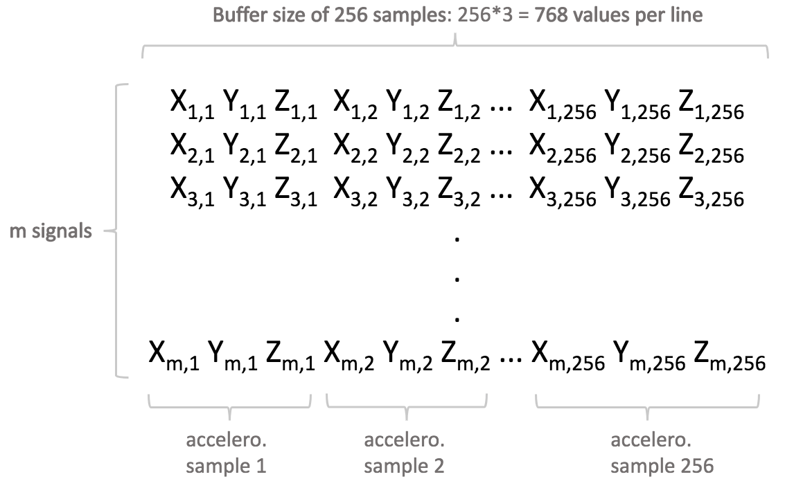
- "buffer size", or "buffer length"; this is the number of samples per signal. For example, a 3-axis signal with buffer length 256 will be represented by 768 (256*3) numerical values.
3.2. Types of projects in NanoEdge AI Studio
The 4 different types of projects that can be created using the Studio, along with their characteristics, outputs, and possible use cases, are outlined below:
Anomaly Detection (AD):
- Use case: detecting anomalies in data using a dynamic model.
- User input: signal examples representing both nominal states and abnormal states (used for library selection only).
- Studio output: untrained anomaly detection library that will learn incrementally, directly on the target microcontroller.
1-class Classification (1CC):
- Use case: detecting anomalies in data using a static model.
- User input: signal examples representing normal states only (used for both library selection and model training).
- Studio output: pre-trained outlier detection library that will infer directly on the target microcontroller.
n-class Classification (nCC):
- Use case: distinguishing among n different states using a static model.
- User input: signal examples representing all the different states (classes) to be expected (used for both library selection and model training).
- Studio output: pre-trained classification library that will infer directly on the target microcontroller.
Extrapolation (EX):
- Use case: estimating an unknown target value using other know parameters, using a static model.
- User input: signal examples associating the know parameters, to their target values (used for both library selection and model training).
- Studio output: pre-trained regression library that will infer directly on the target microcontroller.
3.3. Types of sensors in NanoEdge AI Studio
NanoEdge AI Studio and its output NanoEdge AI Libraries are compatible with any sensor type; they are sensor-agnostic. For example, users may use data coming from an accelerometer, a magnetometer, a microphone, a gas sensor, a time-of-flight sensor, a microphone, or a combination of any of these (list non exhaustive).
The Studio is designed to be able to work with raw sensor data, that hasn't necessarily been pre-processed. However, in cases where users already have some knowledge and expertise about their signals, pre-processed signals can be imported instead.
Depending on the user's use case, the Studio needs to understand which data format to expect in the imported input files. There are 2 main categories of sensors selectable in the Studio:
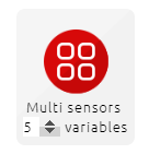
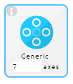
- Generic (n axes) sensor, which is a generalization of some other sensor types, e.g., accelerometer 3 axes, magnetometer 1 axis, microphone (1 axis), current (1 axis), and so on. This sensor covers most typical use cases, and will be selected most of the time.
- Multi-sensor (n variables), referred to as "Multi-sensor", which is specific to anomaly detection projects, and designed for niche use cases, for which the expected format is entirely different.
The Generic n-axis sensor (and all others except "Multi-sensor") expects a buffer of data as input, in other words, a signal example represented by a succession of instantaneous sensor samples. As a result, this "signal example" will have an associated temporal length, which depends on the sampling frequency (output data rate of the sensor) and on the number of instantaneous samples composing the signal example (referred to as buffer size, or buffer length).
The Multi-sensor sensor, on the other hand, expects instantaneous samples of data. In other words, it uses a single sensor sample as input, as opposed to a temporal signal example composed of many samples.
In the remainder of this documentation, except when explicitly stated otherwise, the "Generic" sensor approach (using signal examples / buffers as input, rather that single samples) will be used by default.
3.4. Designing a relevant sampling methodology
Compared to traditional machine learning approaches, which may require hundreds of thousands of signal examples to build a model, NanoEdge AI Studio requires minimal input datasets (as little as 50-100 signal examples, depending on the use case).
However, this data needs to be qualified, which means that it must contain relevant information about the physical phenomena to be monitored. For this reason, it is absolutely crucial to design the proper sampling methodology, in order to make sure that all the desired characteristics from the physical phenomena to be sampled are correctly extracted and translated into meaningful data.
To prepare input data for the Studio, the user must choose the most adequate sampling frequency.
The sampling frequency corresponds to the number of samples measured per second. For some sensors, the sampling frequency can be directly set by the user (e.g. digital sensors), but in other cases (e.g. analog sensors), a timer needs to be set up for constant time intervals between each sample.
The speed at which the samples are taken must allow the signal to be accurately described, or "reconstructed"; the sampling frequency must be high enough to account for the rapid variations of the signal. The question of choosing the sampling frequency therefore naturally arises:
- If the sampling frequency is too low, the readings are too far apart; if the signal contains relevant features between two samples, they are lost.
- If the sampling frequency is too high, it may negatively impact the costs, in terms of processing power, transmission capacity, or storage space for example.
The issues related to the choice of sampling frequency and the number of samples are illustrated below:
- Case 1: the sampling frequency and the number of samples make it possible to reproduce the variations of the signal.

- Case 2: the sampling frequency is not sufficient to reproduce the variations of the signal.

- Case 3: the sampling frequency is sufficient but the number of samples is not sufficient to reproduce the entire signal (meaning that only part of the input signal is reproduced).

The buffer size corresponds to the total number of samples recorded per signal, per axis. Together, the sampling frequency and the buffer size put a constraint on the effective signal temporal length.
Here are general recommendations. Make sure that:
- the sampling frequency is high enough to catch all desired signal features. To sample a 1000 Hz phenomenon, you must at least double the frequency (in this case, sample at 2000 Hz at least).
- your signal is long (or short) enough to be coherent with the phenomenon to be sampled. For example, if you want your signals to be 0.25 seconds long (
L), you must haven / f = 0.25. For example, choose a buffer size of 256 with a frequency of 1024 Hz, or a buffer of 1024 with a frequency of 4096 Hz, and so on.
3.5. Preparing signal files
During the library selection process, NanoEdge AI Studio uses user data (input files containing signal examples) to test and benchmark many signal preprocessing algorithms, Machine Learning models and parameters. The way these input files are structured, formatted, and the way the signal were recorded is therefore very important.
Here are general considerations for input file format, which apply to all cases. The Studio expects:
- .txt / .csv files
- numerical values only (not counting separators), and no headers
- uniform separators throughout the whole file: either
single space,tab,,or;. - decimal values formatted using a period (
.) and not commas (,). - more than 1 sample per line (exception: Multi-sensor)
- fewer than 16384 (214) values per line
- the same number of numerical values on each line
- a bare minimum of 20 lines per sensor axis (e.g. for a 3-axis accelerometer: 60 lines is a bare minimum)
- fewer than ~100000 lines in total (generally, 50-1000 are more than enough)
- file size lower than ~1 Gb
Then, there are some specific formatting rules, mainly depending on the type of project created in the Studio:
- Anomaly detection, 1-class classification, and n-class classification projects all follow the same general rules.
- Extrapolation projects has a particularity, because it needs to incorporate the target values from which to extrapolate.
- Multi-sensor is a big exception, and applies only to niche cases in anomaly detection projects.
3.5.1. General rules
The following applies to anomaly detection (exception: Multi-sensor), 1-class classification, and n-class classification projects.
In NanoEdge AI Studio, lines are taken into account independently, iteratively, so they must represent a meaningful snapshot in time of the signal to be processed. It it therefore crucial to set a coherent sampling frequency and a proper buffer size.
The Studio expects:
- each line to represent a single, independent signal example, made of many samples
- the buffer size of this signal to be a power of two, and to stay constant throughout the project
- the sampling frequency of this signal to stay constant' throughout the project
- all signal examples corresponding to a given "class" to be combined in the same input file (for anomaly detection, it generally means that all "nominal" regimes should be concatenated into a single "nominal" input file, and all "abnormal regimes" into a single "anomalies" input file.
Example:
I am using a 3-axis accelerometer. I want to monitor a piece of equipment that vibrates. I will collect a total of 100 learning examples to represent the vibration behavior of my equipment. I estimate the highest-frequency component of this vibration to be below 500 Hz, therefore I choose a sampling frequency of 1000 Hz for my sensor. I decide that my learning examples for this vibration should represent about 1/4 of a second (250 ms). To achieve this, I choose a buffer size of 256 samples. This means my 256 samples will represent a signal of 1000/256 = 256 ms.
Therefore, in my input file, each signal will be composed of 256 3-value samples. This means each of the 100 lines in my input file will be composed of 768 numerical values (256*3).
3.5.2. Variant: Extrapolation projects
The following applies to extrapolation projects only.
The mathematical models used in NanoEdge AI Extrapolation libraries are regression models (not necessarily linear). Therefore, all general information and rules governing regression apply here.
NanoEdge AI Studio uses input files provided in Extrapolation projects both to find the best possible NanoEdge AI Extrapolation library, and also to train it. It means that the learning examples (lines) provided in the input files should not only contain the signal buffer itself, but also the target values associated to this signal buffer.
The point is to learn a model that will correlate each signal buffer to a target value, so that after training, when it is embedded into the microcontroller, the extrapolation library is able to read a signal buffer, and infer the missing (unknown) target value.
Input file format provided to the Studio for extrapolation only slightly differ from the general guidelines presented in the previous section. The difference is that the signal buffer (each line) should be preceded by a single numerical value, representing the target to evaluate, as shown here:
PLACEHOLDER
PLACEHOLDER
These target values are provided in the Studio for library selection / training, but omitted during testing. Therefore, during testing (e.g. using the NanoEdge AI Emulator), the input file format is exactly the same as the one described in the previous section, titled "General rules".
3.5.3. Exception: Multi-sensor
In anomaly detection projects (only), the Multi-sensor sensor is used to monitor machine "states" that typically evolve slowly in time. These states may be represented by variables coming from distinct sensor sources, and/or result from the aggregation of signal buffers into artificial, higher level features.
Here, the input format is different:
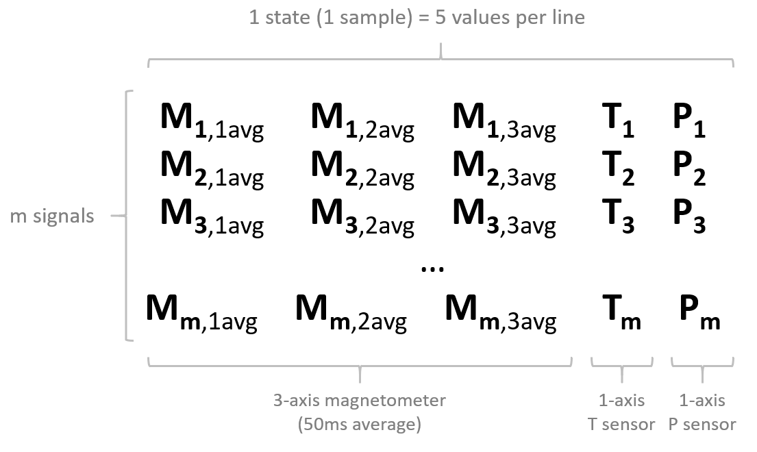
- Each line represents a single sample (possibly multi-variable) instead of a full signal.
- The number of values per line (equal to the number of variables per sample) does not have to be a power of two.
- The lines are not independent, so the ordering does matter (lines should not be shuffled).
- Typically, there are many more lines in the input file compared to the "normal" case (not "Multi-sensor"), since we now have only one sample per line, instead of many samples per line.
Example:
I want to monitor the state of a machine, represented by a combination of sensors; 3-axis magnetometer, a temperature sensor (1 axis), and a pressure sensor (1-axis). Temperature and pressure, if they vary slowly, can be read directly, but magnetometer data needs to be summarized using (for example) average values across a 50 millisecond window along all 3 axes (we do not use instantaneous values). This would result in 3 extracted magnetic features, followed by temperature, followed by pressure, to represent a 5-variable state.
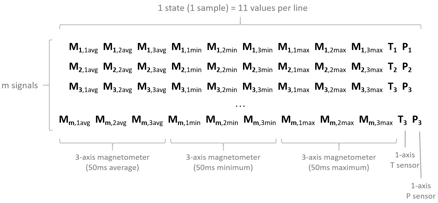
We could also imagine building a more complex state from our 50 millisecond magnetometer buffer, including not only average magnetometer values, but also minima and maxima, for all 3 axes. This would result in 3*3 = 9 extracted magnetometer values (3 each for average, minimum, maximum), followed by temperature and pressure, to represent a 11-variable state.
3.5.4. Which signals to put in which files
For classification, each category of signal examples that wish to be classified / separated must be put into distinct files and imported separately into different "Classes".
For anomaly detection, the general guideline is to concatenate all signal examples corresponding to the same category into the same file (like "nominal").
Example:
I want to detect anomalies on a 3-speed fan by monitoring its vibration patterns using an accelerometer. I recorded many signals corresponding to different behaviors, both "nominal" and "abnormal". I have the following signal examples (numbers are arbitrary):
- 30 examples for "Speed 1", which I consider nominal,
- 25 examples for "Speed 2", which I consider nominal,
- 35 examples for "Speed 3", which I consider nominal,
- 30 examples for "Fan turned off", which I also consider nominal,
- Some of these signals contain "transients", like fan speeding up, or slowing down.
- 30 examples for "fan air flow obstructed at speed 1", which I consider abnormal,
- 35 examples for "fan orientation tilted by 90 degrees", which I consider abnormal,
- 25 examples for "tapping on the fan with my finger", which I consider abnormal,
- 25 examples for "touching the rotating fan with my finger", which I consider abnormal.
Here, I create
- Only 1 nominal input file containing all 120 signal examples (30+25+35+30) covering 4 nominal regimes + transients.
- Only 1 abnormal input file containing all 115 signal examples (30+35+25+25) covering 4 abnormal regimes.
And start a benchmark using only this couple of input files.
4. Using NanoEdge AI Studio
In order to generate a static library, NanoEdge AI Studio walks the user through several steps:
- Creating a new project and setting up its parameters,
- Importing "signal examples" into the studio for context,
- Running the library selection process,
- Testing the best library found by the Studio,
- Compiling and downloading the library [Full version / Featured boards only].
For anomaly detection:
For classification:
4.1. Running NanoEdge AI Studio for the first time
When running NanoEdge AI Studio for the first time, you are prompted for:
- Your proxy settings: if you are using a proxy, use the settings below, otherwise, click NO.
- Here are the IP addresses that need to be authorized:
Licensing API: Cartesiam API for library compilation: 54.147.158.222 52.178.13.227 54.147.163.93 - 54.144.124.187 - 54.144.46.201 - or via URL: https://api.cryptlex.com:443 or via URL: https://api.nanoedgeaistudio.net (alternatively, https://api.cartesiam.net)
- The port you want to use.
- It can be changed to any port available on your machine (port 5000 by default).
- Your license key.
- If you do not know your license key, log in to the Cryptex licensing platform to retrieve it.
- If you have lost your login credentials, reset your password using the email address used to download NanoEdge AI Studio.
- If you do not know your license key, log in to the Cryptex licensing platform to retrieve it.
4.2. Creating a new project
In the main window, you can:
- Create a new project
- Load an existing project

Projects can be imported from and exported to .zip format:
The 3 projects most recently opened are listed first.
4.2.2. Project creation

- Choose project type: Anomaly detection or Classification:
- Enter name and description;
- Choose the target (microcontroller type);
- Arm® Cortex®-M MCUs currently supported: M0, M0+, M1, M3, M4, M23, M33 and M7.
- Selecting an authorized board enables library download and compilation when using NanoEdge AI Studio TRIAL version.
- Here is the list of the authorized boards currently available:
- STMicroelectronics:
- Choose the maximum amount of RAM allocated to the library (maximum: 10 000 Kbytes);
- (optional) Choose the maximum amount of FLASH allocated to the library;
- Choose the sensor type used to collect data (with the correct number of axes);
- Click CREATE.


4.2.3. Which sensor to use for which case
Single-sensor temporal buffer:
This is the typical single-sensor use case where a signal example is composed of a buffer made out of several samples (such as current, magnetometer, accelerometer, or others) Valid sensors to use would be:
Multi-sensor temporal buffer:
To work with temporal buffers coming from multiple sensors of different types, there are 2 different approaches:
- Separate each sensor signal, and create a library for each one, using Multi-library.
- Each signal is decoupled and treated on its own by a different library. See the Multi-library section. This is very similar to the Single-sensor buffer case above, but this time there is a need to monitor several buffers coming from several sensors, concurrently, in the same device.
- Each signal is decoupled and treated on its own by a different library. See the Multi-library section. This is very similar to the Single-sensor buffer case above, but this time there is a need to monitor several buffers coming from several sensors, concurrently, in the same device.
- Combine all signals into a single buffer, by using a generic N-axis sensor.
- All signals are treated concurrently by the same library. The Machine Learning algorithms build therefore a model based on the combination of these inputs (unlike option #1).
- Example:
- To combine accelerometer (3 axes) + gyroscope (3 axes) + current (1 axis) signals, you would select a generic 7-axis sensor.
- The buffers in the input files are formatted just like a generic 3-axis accelerometer (see this section formatting), but each sample now has 7 variables. Instead of the 3 linear accelerations [X Y Z], the 7-axis sample adds 3 angular accelerations [Gx Gy Gz] from the gyroscope, and 1 current value [C] from the current sensor.
- This would result in 7-axis samples [X Y Z Gx Gy Gz C], meaning that for a buffer size of 256, each line would be composed of 7x256 = 1792 numerical values.
- To combine accelerometer (3 axes) + gyroscope (3 axes) + current (1 axis) signals, you would select a generic 7-axis sensor.

Multi-sensor non-temporal state:
See the Multi-sensor section. This is a niche use case, where machine states need to be monitored at defined intervals. Each state is composed of several "variables" (there is no buffer anymore), possibly coming from sensors of different types.

4.3. Importing signal files
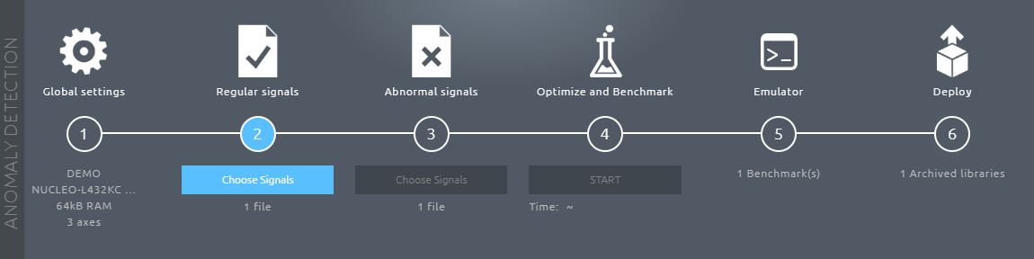
4.3.1. Anomaly detection
For anomaly detection, two types of signals examples are required. They are imported respectively in Step 2: Regular signals and Step 3: Abnormal signals.
- The Regular signals correspond to nominal machine behavior, corresponding to data acquired by sensors during normal use, when everything is functioning as expected.

Include data corresponding to all the different regimes, or behaviors, that you wish to consider as "nominal". For example, when monitoring a fan, you may need to log vibration data corresponding to different speeds, possibly including the transients.
- The Abnormal signals correspond to abnormal machine behavior, corresponding to data acquired by sensors during a phase of anomaly.

The anomalies do not have to be exhaustive. In practice, it would be impossible to predict (and include) all the different kinds of anomalies that could happen on your machine. Just include examples of some anomalies that you've already encountered, or that you suspect could happen. If needed, do not hesitate to create "anomalies" manually. However, if the library is expected to be sensitive enough to detect very "subtle anomalies", it is recommended that the data provided as abnormal signals includes at least some examples of subtle anomalies as well, and not only very gross, obvious ones.
To import a new file, simply click "Choose Signals".
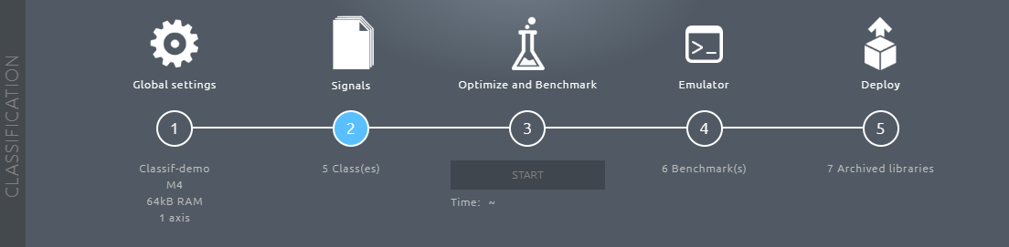
4.3.2. Classification
For classification, you need as many signal types as you have classes to distinguish.
For example, for the identification of types of failures on a motor, 5 classes can be considered, each corresponding to a behavior, such as:
- normal behavior
- misalignment
- imbalance
- bearing failure
- excessive vibration
This would result in the creation of 5 distinct classes (import one .txt / .csv file for each), each containing a minimum of 20-50 signal examples of said behavior.

To add a new class, simply click "Add Class" and then "Choose Signals".

4.3.3. Importing signals from file
Make sure that your input files are formatted properly (see Studio: Formatting input files).
- Click Select file, and choose a valid input file.
- Select the separator you are using.
- Validate import.

If your input file is valid, you are able to import it. Otherwise, double-check your data (numerical values, uniform separators, or constant number of samples per line).
Any imported signal can be plotted and displayed by clicking the icon:
Plots can then be saved to .png format.
4.3.4. Importing signals "live" from Serial port (USB)
It is possible to import signals directly within the Studio, by logging it through your computer serial port (USB).
You need a USB data logger in order to do it. For instructions on how to make a simple data logger, check the tutorials: Smart vibration sensor and Smart current sensor, under section Making a data logger.
- Select your Serial / COM port. Refresh if needed.
- Choose your preferred baudrate.
- If needed, select a maximum number of lines to be recorded.
- Click the red "Record" round button to start the data logging.
- Click the grey "Stop" square button to interrupt the logging.
- Choose your delimiter.
- Validate import.

If your data is valid, you are able to import it. Otherwise, double-check your data logger parameters.
The data logged via serial is plotted in real-time at the bottom of the screen:
This serial plotter window can be toggled on/off by clicking the signal icon, above numlerical data preview:
If any error is found during the real-time data logging via serial, a pop-up window appears, letting you delete or edit the lines where issues were detected.

4.3.5. Checks, errors and warnings
Supported file formats are .txt / .csv. Recommended separators are single spaces, commas or semicolons. Make sure that your input file is correctly formatted.
In this example, an input file contains 200 examples of nominal data (200 lines), for a 3-axis accelerometer that uses a buffer size of 256 (which gives 256x3 = 768 numerical values per line).

The "Check for RAM"" and the next 5 checks are blocking, meaning that you need to fix any error in your input file before proceeding further.
Click "Run optional checks"" to scan your input file and run additional checks, for instance. to search for duplicate signals, equal consecutive values, random values, outliers, and others. Failing these additional checks gives warnings that suggest possible modifications on your input files. Click any warning for more information and advice.

4.3.6. Data plots
On the right of the screen, you can see a preview of data contained in your input files.

These graphs show a summary of the data contained in each line of your input files. There are as many graphs as sensor axes.
The graph x-axis corresponds to the columns of your input file. The y-values contain an indication of the mean value of each column (across all lines, or signals), their min-max values, and their standard deviation.
The FFT plots can be displayed by toggling "Show FFT" at the top-right of the graphs.

Several input files can be loaded (shown on the left of the screen, see below), either for "regular" or "abnormal" signals, but only one (for each) at a time is used for library selection.

4.3.7. Frequency filtering
Since v2.1, it is now possible to alter the imported signals by filtering out unwanted frequencies.
Click Advanced settings above the list of imported signals.

In the Advanced settings menu, you may toggle Activate FFT to force the library to include a fast Fourier transform in its signal pre-processing step. The library treats imported signals in the frequency domain rather than the time domain.

- Input the sampling frequency used to collect your signals (here 6660 Hz)
- Select the range of frequencies to exclude (meaning that everything is excluded under 500 Hz and above 2000 Hz)
- Validate
The FFT plots of your signals are displayed under signal previews, with greyed out zones corresponding to the excluded frequencies (below, only the frequencies between 500 Hz and 2000 Hz are kept).

4.4. Running the library selection process
Here (Step: Optimize and Benchmark), you start and monitor the library benchmark. NanoEdge AI Studio searches for the best possible library given the contextual signal examples provided in the previous step(s).

4.4.1. Starting the benchmark
Click START to open the signal selection window:
[Anomaly detection]:
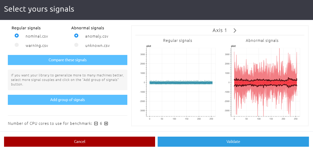
Select a couple of signal files (regular + abnormal signals) that you wish to use for benchmark.
Those signals can be compared visually across all sensor axes by clicking Compare these signals.


[Classification]:
Select the classes to take into consideration for benchmarking.
Then, select the number of microprocessor cores from your computer that you wish to dedicate to the benchmark process (see below). Selecting more CPU cores parallelizes the workload of algorithms, and greatly speed up the process. Use as many as you can, but be aware that using all available CPU cores might temporarily slow down your computer performance.
When you are ready to start the benchmark, click Validate.
4.4.2. Library performance indicators
NanoEdge AI Studio uses 3 indicators to translate the performance and relevance of candidate libraries, in the following order of priority:
- (Balanced) accuracy (most important by far)
- Confidence
- RAM
- Fèlash memory

| Balanced Accuracy (anomaly detection) | Accuracy (classification) |
|
|
| Optimizing this indicator is the top priority of the algorithms. |
| Confidence (anomaly detection) | Confidence (classification) |
|
|
| Increasing this indicator is the algorithms' second priority. |
| RAM and Flash memory (anomaly detection and classification) |
|
This is the maximum amount of RAM and Flash memory space needed by the library after your integrate it on your microcontroller. |
| The amounts of Flash memory and RAM used by the libraries are optimized last. |
Along with those 3 indicators, a graph shows a plot of all data points, against a percentage of similarity (on the y-axis). Similarity is a measure of the how much a given data point fits in with (how much it resembles) the existing knowledge base of the library.
[Anomaly detection]:
Regular signals are shown as blue dots, and abnormal signals as red dots. The x-axis represents the number of the signal example in the corresponding file, and the y-axis represents the similarity score (%). The threshold (decision boundary between the two classes, "nominal" and "anomaly") set at 90% similarity, is shown as a gray dashed line.

For example:
- The blue dot below refers to a signal from the imported "nominal signals" input file, and it is ranked at 67% similarity. It is (incorrectly) detected as anomaly.
- The red dot below refers to a signal from the imported "abnormal signals" input file, and it is ranked at 60% similarity. It is (correctly) detected as anomaly.


[Classification]:
The graph is subdivided into sections, one for each class. The x-axis shows the number of the signal example in the corresponding class file, while the y-axis represents the probability associated to this signal (the % certainty associated to the class detected).
All signal examples are represented as dots, either green if their associated probability is higher than 50%, or red otherwise.

For example:
- The red dot below, pertaining to the class / input file "Obstructed" was (incorrectly) classified as "Nominal".
- All other dots (green) were correcly identified as their respective classes.

4.4.3. Benchmark progress and summary
As soon as the library selection process is initiated, a graph is displayed on the right hand side of the screen (see below), showing the evolution of the 3 performance indicators (see above section) over time, as thousands of candidate library are tested.

The selection algorithms first try to maximise balanced accuracy, then confidence, and finally to decrease the RAM / Flash memory needed as much as possible.


While a benchmark is running, a small log window displays notable information / events such as benchmark status, search speed per thread, and new libraries found.

When the benchmark is complete, the progress graph is be replaced by a summary.


Several successive benchmarks can be run; all results are saved. They can be loaded by clicking them on the left hand side of the screen.

[Anomaly detection only]: After the benchmark is complete, a plot of the library learning behavior is shown:

This graph shows the number of learning iterations needed to obtain optimal performance from the library, when it is embedded in your final hardware application. In this particular example, NanoEdge AI Studio recommended that the learn() is called 70 times, at the very minimum.
4.4.4. Possible cause for poor benchmark results
If your keep getting poor benchmark results, you may try the following:
- Increase the "Max RAM" or "Max Flash"" parameters (such as 32 Kbytes or more).
- Adjust your sampling frequency; make sure it is coherent with the phenomenon you want to capture.
- Change your buffer size (and hence, signal length); make sure it is coherent with the phenomenon to sample.
- Make sure your buffer size (number of values per line) is a power of two (except for multi-sensor).
- If using a multi-axis sensor, treat each axis individually by running several benchmarks with a single-axis sensor.
- Include more signal examples (lines) in your input files.
- Check the quality of your signal examples; make sure they contain the relevant features / characteristics.
- Check that your input files do not contain (too many) parasite signals (for instance no anomalous signals in the nominal file, for anomaly detection, and no signals belonging to another class, for classification).
- Increase the variety of your signal examples (more nominal regime, or more anomalies, or more classes).
- Decrease the variety of your signal examples ( fewer nominal regime, or fewer anomalies, or fewer classes).
- Check that the sampling methodology and sensor parameters are kept constant throughout the project for all signal examples recorded (in all input files; nominal, abnormal or class files).
- Check that your signals are not too noisy, too low intensity, too similar, or unrepeatable.
- Remember that microcontrollers are resource-constrained (audio/video, image and voice recognition are not be supported).
Low confidence scores are not necessarily an indication or poor benchmark performance, if the (balanced) accuracy is sufficiently high (> 80-90%). Always use the associated Emulator to determine the performance of a library, preferably using data that has not been used before (for the benchmark).
4.5. Testing the NanoEdge AI Library
Here (Step: Emulator), you are able to test the library that was selected during the benchmark process (Step: Optimize and Benchmark) using NanoEdge AI Emulator.

NanoEdge AI Emulator is a clone of the library that emulates its behavior, and is directly usable within the Studio interface. There is no need to embed a library in order to test its performance with real, "unseen" data. Therefore, each library, among hundreds of thousands of possibilities, comes with its own Emulator.
The Emulator can be also be downloaded as a standalone .exe (Windows®) or .deb (Linux®) to be used in the terminal through the command line interface.
This screen gives a summary of the selected benchmark (progress, performance, input files used):
Select the benchmark to use, on the left side of the screen, to load the associated emulator.
When you are ready to start testing, click Initialize Emulator.
4.5.1. Anomaly detection
Functions:
Here are the functions of the anomaly detection library that are available through its Emulator:
initialize()
|
run first before learning/detecting, or to reset the knowledge of the library/emulator |
set_sensitivity()
|
adjust the pre-set, internal detection sensitivity (does not affect learning, only returned similarity scores) |
learn()
|
start a number of learning iterations (to establish an initial knowledge, or enrich an existing one) |
detect()
|
start a number detection iterations (inference), once a minimum knowledge base has been established |
For more information, see the Emulator and Library documentations for anomaly detection.
The testing procedure goes as follows:

Learning:
After initialization, no knowledge base exists yet. It needs to be acquired in-situ, using real signals. Your library is not pre-trained with the signals imported before benchmark, in Steps 2 and Step 3. Therefore, you need to learn some signals.
To learn some signals from a file, click Select file and open the file containing your training data.
To learn some signals "live" from your Serial port, using your own data logger, click Serial data. Then, select your Serial / COM port (refresh if needed), choose your preferred baudrate, and Start recording by clicking the red button.
As soon as some signals are learned, the number of learned signals is indicated.
Click Go to detection after all relevant signals (nominal, by definition) have been learned.
Detection:
When a first knowledge base has been established, you can use Detection using any signals, to check if they would be classified as nominal or anomaly by the library, and make sure this library performs as intended.
As usual, the signals to use for detection can be imported from file, or from Serial port using a data logger.
Select the signals that you wish to use, and adjust the sensitivity if needed. A pie chart summarizes the detection results.
When detecting using live data from the Serial port, a graph shows how the detection performance (similarity percentage) evolves in real time.

4.5.2. Classification
Here are the functions of the classification library that are available through its Emulator:
knowledge_init()
|
run first to initialize the knowledge |
classifier()
|
run an inference iteration (detect which class the input signal belongs to) |
For more information, see the Emulator and Library documentations for classification.
Just like in anomaly detection (see "Important" section above), the classifier function can be called dynamically whenever needed. It can be triggered by external data (for example from sensors, buttons, to account for and adapt to environment changes), and the class / probabilities returned can trigger all kinds of behaviors on your device.
To classify signals from a file, click Select file and open the file containing the signal examples to classify. You can see a pie chart summarizing the classification.
The image below shows data from a 3-speed fan:
- 3 signals were detected at "speed 1"
- 7 at "speed 2"
- 17 at "speed 3"
- 6 when the fan air flow was obstructed
- and so on

You see a pie chart summarizing the classification, as well as a graph showing the probabilities associated to each classification iteration (the image below shows data from a 3-speed fan, and "speed 1" is currently being detected).


4.5.3. Possible causes of poor emulator results
Here are possible reasons for poor anomaly detection or classification results:
- The data used for library selection (benchmark) is not coherent with the one you are using for testing via Emulator/Library. The regular/abnormal or class signals imported in the Studio must correspond to the same machine behaviors, regimes, and physical phenomena as the ones used for testing.
- Your (balanced) accuracy score was well below 90% or your confidence score was too low to provide sufficient data separation.
- You used an insufficient number or signals in either regular/abnormal or class signal files. Make sure that you used enough lines in your input files (minimum 20-50). For anomaly detection, make sure that you use at least the minimum number recommended by the Studio, and possibly more.
- The sampling method is inadequate for the physical phenomena studied, in terms of frequency, buffer size, or duration for instance.
- The sampling method has changed between Benchmark and Emulator tests. The same parameters (frequency, signal lengths, buffer sizes) must be kept constant throughout the whole project.
- [Anomaly detection]: you have not run enough learning iterations (your Machine Learning model is not rich enough), or this data is not representative of the signal examples used for benchmark. Do not hesitate to run several learning cycles, as long as they all use nominal data as input (only normal, expected behavior should be learned).
- [Classification]: the machine status or working conditions have drifted between Benchmark and Emulator tests, and classes are not recognized anymore. In that case, update the imported "class" files, and start a new benchmark.
4.6. Downloading the NanoEdge AI Library
This feature is only available:
- in the Trial version of NanoEdge AI Studio, limited to the featured boards which can be selected during project creation
- in the Paid version of NanoEdge AI Studio
4.6.1. General case
In this step (Step: Deploy), the library is compiled and downloaded, ready to be used on your microcontroller for your embedded application.

Before compiling the library, several compilation flags are available:
- [[File:NanoEdgeAI_compilation_flags.png]
If you ran several benchmarks, make sure that the correct benchmark is selected. Then, when you are ready to download the NanoEdge AI Library, click Compile.
Select Development version to get a library that is intended for testing and prototyping. If you would like to start producing your device, integrating NanoEdge AI Library, contact STMicroelectronics for more details and to get the proper library version.
After a short delay, a .zip file is downloaded to your computer.

It contains all relevant documentation, the NanoEdge AI Emulator (both Windows® and Linux® versions), the NanoEdge AI header file (C and C++), a .json file containing some library details, and the model knowledge (for classification only).
You can also re-download any previously compiled library, via the archived libraries list:

4.6.2. Multi-library
In this final step (Step: Deploy) you also have the possibility to add a suffix to the library you are about to compile and download.

This is useful to integrate multiple libraries into the same device / code, when there is a need to:
- monitor several signal sources coming from different sensor types, concurrently, independently,
- train Machine Learning models and gather knowledge from these different input sources,
- take decisions based on the outputs of the Machine Learning algorithms for each signal type.
For instance, one library can be created for 3-axis vibration analysis, and suffixed vibration:
Later on, a second library can be created later on, for 1-axis electric current analysis, and suffixed current:
All the NanoEdge AI functions in the corresponding libraries (as well as the header files, variables, and knowledge files if any) is suffixed appropriately, and is usable independently in your code. See below the header files and the suffixed functions and variables corresponding to this example:

Congratulations! You can now use your NanoEdge AI Library!
It is ready to be linked to your C code using your favorite IDE, and embedded in your microcontroller.
For more info, check the library documentation (AD library, CL library), as well as the code snippets on the right side of the screen, which provide general guidelines about how your code could be structured, and how the NanoEdge AI Library functions must be called.
5. Resources
Documentation
All NanoEdge AI Studio documentation is available here.
Tutorials
Step-by-step tutorials, to use NanoEdge AI Studio to build a smart device from A to Z.