NanoEdge AI Studio

This message will disappear after all relevant tasks have been resolved.

Semantic MediaWiki

There are 1 incomplete or pending task to finish installation of Semantic MediaWiki. An administrator or user with sufficient rights can complete it. This should be done before adding new data to avoid inconsistencies.

NanoEdge AI Studio is a free software provided by ST to easily add AI into to any embedded project running on any Arm © Cortex M MCU.

It empowers embedded engineers, even those unfamiliar with AI, to almost effortlessly find the optimal AI model for their requirements through straightforward processes.

Operated locally on a PC, the software takes input data and generates a NanoEdge AI library that incorporates the model, its preprocessing, and functions for easy integration into new or existing embedded projects.

The main strength of NanoEdge AI Studio is its benchmark which will explore thousands of combinations of preprocessing, models and parameters. This iterative process identifies the most suitable algorithm tailored to the user's needs based on their data.

1. Getting Started

1.1. What is NanoEdge AI Studio?

NanoEdge AI Studio is a software designed for embedded machine learning. It acts like a search engine, finding the best AI libraries for your project. It needs data from you to figure out the right mix of data processing, model structure, and settings.

Once it finds the best setup for your data, it creates AI libraries. These libraries make it easy to use the data processing and model in your C code.

1.1.1. NanoEdge AI Library

NanoEdge™ AI Libraries are the output of NanoEdge AI Studio. They are static library for embedded C software on Arm® Cortex® microcontrollers (MCUs). Packaged as a precompiled .a file, it provides building blocks to integrate smart features into C code without requiring expertise in Mathematics, Machine Learning, or data science.

When embedded on microcontrollers, the NanoEdge AI Library enables them to automatically "understand" sensor patterns. Each library contains an AI model with easily implementable functions for tasks like learning signal patterns, detecting anomalies, classifying signals, and extrapolating data.

Each kind of project in NanoEdge has it own kind of AI Library with their functions but they share the same characteristics:

Highly Optimized: Designed for MCUs (any Arm® Cortex®-M).
Memory Efficient: Requires only 1-20 Kbytes of RAM/flash memory.
Fast Inference: Executes in 1-20 ms on Cortex®-M4 at 80 MHz.
Cloud Independent: Runs directly within the microcontroller.
Easy Integration: Can be embedded into existing code/hardware.
Energy Efficient: Minimal power consumption.
Static Allocation: Preserves the stack.
Data Privacy: No data transmission or saving.
User-Friendly: No Machine Learning expertise required for deployment.

All NanoEdge AI Libraries are created using NanoEdge AI Studio.

1.1.2. Nanoedge AI Studio Capabilities

NanoEdge AI Studio can:

Search for optimal AI libraries (preprocessing + model) given user data.
Simplify the development of machine learning features for embedded developers.
Minimize the need for extensive machine learning and data science knowledge.
Utilize minimal input data compared to traditional approaches.

Using project parameters (MCU type, RAM, sensor type) and signal examples, the Studio outputs the most relevant NanoEdge AI Library. This library can be either untrained (learning post-embedding) or pre-trained. The library performs inference directly on the microcontroller, involving:

Signal preprocessing algorithms (e.g., FFT, PCA, normalization).
Machine learning models (e.g., kNN, SVM, neural networks, proprietary algorithms).
Optimal hyperparameter settings.

The process is iterative: import signals, run a benchmark, test the library, adjust data, and repeat to improve results.

1.1.3. Nanoedge AI Studio Limitations

NanoEdge AI Studio:

Requires user-provided input data (sensor signals) for satisfactory results.
Libraries' performances are heavily correlated to the quality of the data imported
Does not offer ready-to-use C code for final implementation. Users must write, compile, and integrate the code with the AI library.

In summary, NanoEdge AI Studio outputs a static library (.a file) based on user data, which must be linked and compiled with user-written C code for the target microcontroller.

1.2. License Activation

To use NanoEdge AI Studio, you need a license obtained during the software download at stm32ai.st.com.

Initial Setup

Enter your license key
Set your proxy settings if you need
Save Settings

IP Authorization You may need to authorize the following IP addresses:

ST API for library compilation:	52.178.13.227	or via URL: https://api.nanoedgeaistudio.net

Port Configuration

By default, NanoEdge AI Studio uses port 5000. If this port is unavailable, the Studio will automatically search for an available port. To manually configure the port:

Press windows key + R, type %appdata% and press Enter.
Navigate to nanoedgeaistudio folder and open config.json
Locate the line where the port is set, modify it, and save the file.

Project Storage Location You can change the location where projects are saved. Avoid selecting cloud-synced or shared folders for project storage.

1.2.1. Offline license activation

If you lack an Internet connection, you can activate your NanoEdge AI Studio license offline:

Offline Activation: Click on "Offline Activation" and enter your license key.
Copy the Activation String: A long string of characters will appear. Copy this string or click the provided link.
Activate License: Paste the string if needed and click "Activate License".
Receive Response String: You will receive a new string as a response. Copy this string.
Finalize Activation: Return to NanoEdge AI Studio, paste the response string, and click "Activate".

1.3. Type of projects

The four different types of projects that can be created using the Studio, along with their characteristics, outputs, and possible use cases, are outlined below:

Anomaly detection differentiates normal behavior signals from abnormal ones.

User Input: Datasets containing signals for both normal and abnormal situations.
Studio Output: The optimal anomaly detection AI library, including preprocessing and the model identified during benchmarking.
Library Output: The library provides a similarity score (0-100%) indicating the resemblance between the training data and the new signal.
Retraining: This project type supports model retraining directly on the microcontroller. [More information here].
C Library Functions: Includes initialization, learning, and detection functions. [More details here].
Use Case Example: For preventive maintenance of multiple machines, collect nominal data and simulate possible anomalies. Use NanoEdge AI Studio to create a library that can distinguish normal and abnormal behaviors. Deploy the same model on all machines and retrain it for each specific machine to enhance specialization for their environments.

Important

Anomaly detection is the only project type that outputs a NanoEdge AI Library capable of learning signal examples in situ, after it is embedded into the microcontroller. All other library types only infer in the microcontroller.

This feature gives anomaly detection libraries great adaptability, since the same library, deployed on different devices (possibly monitoring slightly different machines, or machines that operate in different environmental conditions, or that are susceptible to perturbations) is able to train differently (learn different knowledge) to adapt itself to the specific behavior of its target machine.

This also means that anomaly detection libraries can learn incrementally on the go; knowledge can be erased, but it can also be enriched at any moment, simply by learning additional signal examples representing the new behaviors to learn (for instance signals representing new nominal regimes, possibly due to a change in operating conditions).

N-class classification assigns a signal to one of several predefined classes based on training data.

User Input: A dataset for each class to be detected.
Studio Output: The optimal N-class classification library, including preprocessing and the model identified during benchmarking.
Library Output: The library produces a probability vector corresponding to the number of classes, indicating the likelihood of the signal belonging to each class. It also directly identifies the class with the highest probability.
C Library Functions: Includes initialization and classification functions. [More details here].
Use Case Example: For machines prone to various errors, use N-class classification to precisely identify the type of error occurring, rather than just detecting the presence of an issue.

One-class classification distinguishes normal behavior from abnormalities without needing abnormal examples, detecting outliers instead.

User Input: A dataset containing only nominal (normal) examples.
Studio Output: The optimal one-class classification library, including preprocessing and the model identified during benchmarking.
Library Output: The library returns 0 for nominal signals and 1 for outliers.
C Library Functions: Includes initialization and detection functions. [More details here].
Use Case Example: For predictive maintenance when abnormal data is unavailable, one-class classification can identify outliers. However, for better performance, using anomaly detection is recommended.

Extrapolation predicts discrete values, commonly known as regression.

User Input: A dataset containing pairs of target values to predict and corresponding signals. Data format differs from other projects in NanoEdge. [See here for details].
Studio Output: The optimal extrapolation library, including preprocessing and the model identified during benchmarking.
Library Output: The library predicts the target value based on the input signal.
C Library Functions: Includes initialization and prediction functions. [More details here].
Use Case Example: When monitoring a machine with multiple sensors, use extrapolation to predict the value of one sensor using data from other sensors. Create a dataset with signals representing the data evolution from the sensor to be kept and associate it with the values from the sensor to be replaced.

1.4. Data format

1.4.1. Defining important concepts

Here are some clarifications regarding important terms that are used in this document and in NanoEdge:

Axis/Axes:
In NanoEdge AI Studio, the axis/axes are the total number of variables outputted by the sensor used for a project. For example, a 3-axes accelerometer outputs a 3-variables sample (x,y,z) corresponding to the instantaneous acceleration measured in the 3 spatial directions.

In case of using multiple sensors, the number of axes is the total number of axes of all sensors. For example, if using a 3-axes accelerometer and a 3-axes gyroscope, the number of axes is 6.

Signal:
A signal is the continuous representation in time of a physical phenomenon. We are sampling a signal with a sensor to collect samples (discrete values). Example: vibration, current, sound.

Sample:
This refers to the instantaneous output of a sensor, and contains as many numerical values as the sensor has axes. For example, a 3-axis accelerometer outputs 3 numerical values per sample, while a current sensor (1-axis) outputs only 1 numerical value per sample.

Data rate:
The data rate is the frequency at which we capture signal values (samples). The data rate must be chosen according to the phenomenon studied. You must also pay attention to having a consistent data rate and number of samples to have buffers that represent a meaningful time frame.

Buffer:
A buffer is a concatenation of consecutive samples collected by a sensor. A dataset contains multiples buffers, the term Line is also used when talking about buffers of a dataset. Buffers are the input for NanoEdge, being in the Studio or in the microcontroller.

1.4.2. General rules

NanoEdge AI Studio expects buffers and not just samples of data.

Buffer = number of axes * number of sample taken at a fixed data rate (Hz)
It's crucial to maintain a consistent sampling frequency and buffer size.

In machine learning, you want to work on buffer as they contains information on the evolution of the phenomenon studied. Samples are just a single point in time representing the phenomenon. It is easier to distinguish pattern in buffers than in simple value.

The Studio requires:

Each line in a dataset must represent a single, independent signal example composed of multiple samples.
The buffer size to be a power of two and remain constant throughout the project.
The sampling frequency to remain constant throughout the project.
All signal examples for a specific "class" to be grouped in the same input file (e.g., all "nominal" regimes in one file and all "abnormal" regimes in another for anomaly detection).

General considerations for input file format:

.txt / .csv files
Numerical values only, no headers
Uniform separators (single space, tab, comma, or semicolon)
Decimal values formatted with a period (.)
More than 1 sample per line (except Multi-sensor)
Fewer than 16,384 values per line
Consistent number of numerical values on each line
Minimum of 20 lines per sensor axis
Fewer than ~100,000 total lines
File size less than ~1 Gbit

Specific formatting rules:

Anomaly detection, 1-class classification, and n-class classification projects share general rules.
Extrapolation projects require target values for extrapolation.

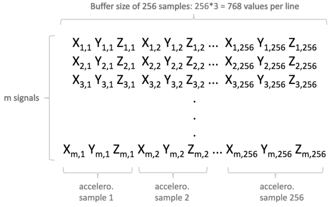
1.4.3. Basic Format

Example:

I am using a 3-axis accelerometer. I want to monitor a piece of equipment that vibrates. I will collect a total of 100 learning examples to represent the vibration behavior of my equipment. I estimate the highest-frequency component of this vibration to be below 500 Hz, therefore I choose a sampling frequency of 1000 Hz for my sensor. I decide that my learning examples for this vibration represent about 1/4 of a second (250 ms). To achieve this, I choose a buffer size of 256 samples. This means my 256 samples will represent a signal of 256/1000 = 256 ms.

Therefore, in my input file, each signal will be composed of 256 3-value samples. This means each of the 100 lines in my input file will be composed of 768 numerical values (256*3).

Information

Depending on project constraints, buffer size, signal lengths, and sampling frequencies vary.
For example, for a buffer size of 256, it can mean that:

the capture of 0.25-second signals, with a sampling frequency of 1 kHz implied the choice of a buffer size of 256 (256/1000 = 0.256).
the sampling at a higher frequency (4 kHz), so with a buffer size of 256, led to much shorter signals, 64 ms (256/4000 = 0.064).

1.4.4. Variant Froamt: Extrapolation projects

The following applies to extrapolation projects only.

The mathematical models used in NanoEdge AI Extrapolation libraries are regression models (not necessarily linear). Therefore, all general information and rules governing regression apply here.

NanoEdge AI Studio uses input files provided in extrapolation projects both to find the best possible NanoEdge AI Extrapolation library, and also to train it. It means that the learning examples (lines) provided in the input files must not only contain the signal buffer itself, but also the target values associated to this signal buffer.

The point is to learn a model that correlates each signal buffer to a target value, so that after training, when it is embedded into the microcontroller, the extrapolation library is able to read a signal buffer, and infer the missing (unknown) target value.

Important

Here, the buffer refers to the combination of all known parameters or features associated to a target value. The target value refers to the variable or feature that the user is trying to extrapolate / infer / evaluate / predict. This target value is known during training (hence provided in the input files provided in the Studio), but unknown during inference (hence absent from the input files used later on to test the extrapolation library obtained).

Input file format provided to the Studio for extrapolation only slightly differ from the general guidelines presented in the previous section. The difference is that the signal buffer (each line) must be preceded by a single numerical value, representing the target to evaluate, as shown here:

Warning

These target values are provided in the Studio for library selection / training, but omitted during testing.
Therefore, during testing (for instance when using the NanoEdge AI Emulator), the input file format is exactly the same as the one described in the previous section, titled General rules.

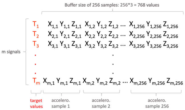
Example:

I am trying to evaluate / predict / extrapolate my running speed (which is my target value) from raw 3-axis accelerometer data.

I choose a sampling frequency of 500 Hz on my accelerometer (which I believe will be sufficient to capture all vibratory characteristics or my "running signature"), and a buffer size of 1024 (because at 500 Hz it will represent a temporal signal segment of approximately 2 seconds, which I estimate will contain sufficient information to extrapolate a speed).
I also need a way to measure my running speed (target value), in order to train the model later on. For instance, I can use a (GPS) speedometer, or simply run a known distance and record my time.
Then, I can start collecting data.
I will walk / run several times while carrying my speedometer and accelerometer, to collect both accelerometer buffers and the associated speeds.
For instance, I will walk / run 6 times, at 6 noticeably different speeds, each time for 1 minute at constant speed. Therefore, for each run, I will get one known speed value, and many (approximately 30) two-second accelerometer buffers composed of 1024*3 = 3072 values each.
Finally, I compile this data in a single file that I will use as input in the Studio.
- This file contains approximately 180 lines (6 runs with 30 buffers each), each representing an individual training example.
- Each line is composed of 3073 numerical values: 1 speed value followed by 1024*3 accelerometer values, all separated (for example) by commas.
- The first 30 lines all start with the same speed value, but have different associated accelerometer buffers (1st run). The 30 next lines all start with another speed value, and have their associated accelerometer buffers (2nd run), and so on.
After my model is trained, I am able to evaluate my running speed, just by providing the best NanoEdge AI library found by the Studio, with some accelerometer buffers of size 1024 sampled at 500 Hz (of course, without providing the speed value). The data provided for inference (or testing) therefore contains 3072 values only (no speed), since speed is what I am trying to estimate.

1.4.5. Designing a relevant sampling methodology

Recommended resource: NanoEdge AI Datalogging MOOC.

Compared to traditional machine learning approaches, which might require hundreds of thousands of signal examples to build a model, NanoEdge AI Studio requires minimal input datasets (as little as 50-100 signal examples, depending on the use case).

However, this data needs to be qualified, which means that it must contain relevant information about the physical phenomena to be monitored. For this reason, it is absolutely crucial to design the proper sampling methodology, in order to make sure that all the desired characteristics from the physical phenomena to be sampled are correctly extracted and translated into meaningful data.

To prepare input data for the Studio, the user must choose the most adequate sampling frequency.

The sampling frequency corresponds to the number of samples measured per second. For some sensors, the sampling frequency can be directly set by the user (such as digital sensors), but in other cases (such as analog sensors), a timer needs to be set up for constant time intervals between each sample.

The speed at which the samples are taken must allow the signal to be accurately described, or "reconstructed"; the sampling frequency must be high enough to account for the rapid variations of the signal. The question of choosing the sampling frequency therefore naturally arises:

If the sampling frequency is too low, the readings are too far apart; if the signal contains relevant features between two samples, they are lost.
If the sampling frequency is too high, it might negatively impact the costs, in terms of processing power, transmission capacity, or storage space for example.

Important

To help you select a good sampling rate and data length please look at the sampling finder

To choose the sampling frequency, prior knowledge of the signal is useful in order to know its maximum frequency component. Indeed, to accurately reconstruct an output signal from an input signal, the sampling frequency must be at least twice as high as the maximum frequency that you wish to detect within the input signal.

Without any prior knowledge of the signal, it is recommended to test several sampling frequencies and refine them according to the results obtained via NanoEdge AI Studio / Library (such as 200 Hz, 500 Hz, 1000 Hz, or others).

The issues related to the choice of sampling frequency and the number of samples are illustrated below:

Case 1: the sampling frequency and the number of samples make it possible to reproduce the variations of the signal.

Case 2: the sampling frequency is not sufficient to reproduce the variations of the signal.

Case 3: the sampling frequency is sufficient but the number of samples is not sufficient to reproduce the entire signal (meaning that only part of the input signal is reproduced).

The buffer size corresponds to the total number of samples recorded per signal, per axis. Together, the sampling frequency and the buffer size put a constraint on the effective signal temporal length.

Important

In summary, there are three important parameters to consider:

n: buffer size
f: sampling frequency
L: signal temporal length

They are linked together via: n = f * L. In other words, by choosing two (according to your use case), the third one is constrained.

(And Signal length = n * number of axis)

Information

For Multi-sensor, the concept of "buffer size" is not relevant, since there are only individual samples in the input files imported in the Studio, instead of full signal examples made of a collection of samples.

Here are general recommendations. Make sure that:

the sampling frequency is high enough to catch all desired signal features. To sample a 1000 Hz phenomenon, you must at least double the frequency (in this case, sample at 2000 Hz at least).
your signal is long (or short) enough to be coherent with the phenomenon to be sampled. For example, if you want your signals to be 0.25 seconds long (L), you must have n / f = 0.25. For example, choose a buffer size of 256 with a frequency of 1024 Hz, or a buffer of 1024 with a frequency of 4096 Hz, and so on.

Information

For best performance, always use a buffer size n that is a power of two (for instance 128, 512 or others).

2. Using NanoEdge AI Studio

2.1. Studio home screen

The Studio main (home) screen has four main elements:

1. Project Creation Bar (top): Create new projects (anomaly detection, 1-class classification, n-class classification, or extrapolation), and access the datalogger and data manipulation screens.

2. Existing Projects List (left side): Load, import/export, or search existing NanoEdge AI projects.

3. Useful Links and Inspiration (right side): Access resources like MOOC, documentation, and links to the Use Case Explorer data portal for downloadable datasets and performance summaries.

4. Toolbar (left extremity): Provides quick access to:

Datalogger
Data manipulation
Sampling finder
Studio settings (port, workspace folder path, license information, and proxy settings)
NanoEdge AI documentation
NanoEdge AI license agreement
CLI (command line interface client) download
Studio log files (for troubleshooting)
Studio workspace folder

2.2. Creating a new project

On the main screen, select your desired project type on the project creation bar, and click CREATE NEW PROJECT.

Each project is divided into 5 successive steps:

Project settings, to set the global project parameters
Signals, to import signal examples that are used for library selection.
Note: this step is divided in 2 substeps in anomaly detection projects (Regular signals / Abnormal signals)
Optimize & benchmark, where the best NanoEdge AI Library is automatically selected and optimized
Emulator, to test the candidate libraries before embedding them into the microcontroller
Validation to have a summary of the project benchmarks (data, performance, flows)
Deployment, to compile and download the best library and its associated header files, ready to be linked to any C code.

A helper tool providing tips is available on the bottom right corner of the screen when in a project. We highly recommend to complete the tasks given and read the documentation highlighted by it!

2.2.1. Project settings

The first step in any project is Project settings.

Here, the following parameters parameters are set:

Project name
Description (optional)
Max RAM: this is the maximum amount of RAM memory to be allocated to the AI library. It does not take into consideration the space taken by the sensor buffers.
Limit Flash / No Flash limit: this is the maximum amount of flash memory to be allocated to the AI library.
Sensor type: the type of sensor used to gather data in the project, and the number of axes / variables when using a "Generic" sensor or "Multi-sensor".
Target: this is the type of board or microcontroller on which the final NanoEdge AI Library is deployed.
Look below for more information on the available targets.

Warning

Restricting the amount of RAM/flash memory available restricts the search space during benchmark', which causes potentially better, more memory-hungry libraries, to be ignored.

2.2.1.1. Target selection

NanoEdge AI Studio allows compilation on a large variety of targets. These target are separated in three tabs:

Development boards: 140+ available targets, greats for education or proof of concepts as development board generally embed sensors.

Microcontrollers: 550+ targets
- Any STM32 Arm © Cortex M MCU: All STM32 families with a Arm © Cortex M MCU can be selected as target.
- A large variety of non ST Arm © Cortex M MCUs for development purposes only.

Arduino Boards: 19 targets with Arm © Cortex M MCUs for development purposes only.

For non-ST target and production purposes, please contact ST.

Important

It is possible to change the target at any moment in a project in progress. It only affect the compilation step. It allow an easy transition from a development board to a production board for example. Just make sure that the new selected target has enough RAM and Flash compared to the library selected.

It is possible to add a board as favorite by clicking on the star. Then, the board will always be displayed on the left.

2.2.1.2. Working with multiple sensors

When combining different sensor types together, three distinct approaches can be used:

1. Using the Generic sensor:

The Generic sensor can be used to combine multiple sensor types together into a single, unified signal buffer that is treated by the library as one multi-variable input.
The Machine Learning algorithms therefore build a model based on the combination of these inputs.
All signal sources must have the same output data rate (sampling frequency).
Example: combining accelerometer (3 axes) + gyroscope (3 axes) + current (1 axis) signals, into a unified 7-axis signal.
- The Generic sensor must be selected, with 7 axes.
- The buffers in the input files are formatted just like a generic 3-axis accelerometer (see the General formatting rules section), but each sample now has 7 variables.
  Instead of the 3 linear accelerations [X Y Z], the 7-axis sample adds 3 angular accelerations [Gx Gy Gz] from the gyroscope, and 1 current value [C] from the current sensor.
- This results in 7-axis samples [X Y Z Gx Gy Gz C], meaning that for a buffer size of 256, each line is composed of 1792 numerical values (7*256).

2. Using the Multi-sensor:

In the same way, Multi-sensor enables the combination of multiple variables into the same library, to be treated as a single, unified input.
All the restrictions related to Multi-sensor regarding input file format apply, see the Multi-sensor formatting section.

3. Using the Multi-library feature (selectable on the Studio Deployment screen):

This approach is radically different, and consists in separating the different sensor types, to create a separate library for each one.
Each signal is decoupled and treated on its own by a different library, that runs concurrently in the same microcontroller. See the Multi-library section.
Here, the output data rates of the different sensors might be different.

2.3. Types of sensors in NanoEdge AI Studio

NanoEdge AI Studio and its output NanoEdge AI Libraries are compatible with any sensor type; they are sensor-agnostic. For example, users can use data coming from an accelerometer, a magnetometer, a microphone, a gas sensor, a time-of-flight sensor, a microphone, or a combination of any of these (list non exhaustive).

The Studio is designed to be able to work with raw sensor data that has not necessarily been pre-processed. However, in cases where users already have some knowledge and expertise about their signals, pre-processed signals can be imported instead.

Depending on the user's use case, the Studio needs to understand which data format to expect in the imported input files. There are 2 main categories of sensors selectable in the Studio:

Generic (n axes) sensor, which is a generalization of some other sensor types, such as accelerometer 3 axes, magnetometer 1 axis, microphone (1 axis), current (1 axis), and so on. This sensor covers most typical use cases, and is selected most of the time.
Multi-sensor (n variables), referred to as "Multi-sensor", which is specific to anomaly detection projects, and designed for niche use cases, for which the expected format is entirely different.

The Generic n-axis sensor (and all others except "Multi-sensor") expects a buffer of data as input, in other words, a signal example represented by a succession of instantaneous sensor samples. As a result, this "signal example" has an associated temporal length, which depends on the sampling frequency (output data rate of the sensor) and on the number of instantaneous samples composing the signal example (referred to as buffer size, or buffer length).

Important

This Generic sensor approach is the main approach, to be used by default, since it covers all possible sensor types (and combinations), all project types, and most use cases.

It is especially relevant when the physical phenomena sampled evolve "quickly" (such as accelerometer, current sensor, and so on), using output data rates higher anywhere above a few hertz (for example, 10 Hz to 20 000 Hz).

The Multi-sensor sensor, on the other hand, expects instantaneous samples of data. In other words, it uses a single sensor sample as input, as opposed to a temporal signal example composed of many samples.

Important

This Multi-sensor, only available in anomaly detection projects, is typically used when the physical phenomena sampled evolve "slowly" over time (such as temperature, pressure or others), or when they do not explicitly depend on time. A typical use case for this sensor is the monitoring of artificial "machine states" represented by signals forming higher-level features, resulting from the aggregation of multiple variables, possibly coming from multiple sensors. Such signals therefore represent instantaneous states rather than time-evolving signals.

In the remainder of this documentation, except when explicitly stated otherwise, the "Generic" sensor approach (using signal examples / buffers as input, rather than single samples) is used by default.

2.3.1. Signals

2.3.1.1. How to import signals

The input files, containing all the signal examples to be used by the Studio to select the best possible AI library, can be imported from three sources:

From a file (in .txt / .csv format)
From the serial port (USB) of a live datalogger
From the FP-SNS-Datalog

1. From file:

Click SELECT FILES, and select the input file to import.
Rename the input file if needed.
Repeat the operation to import more files.
Click CONTINUE.

2. From serial port:

Select the COM Port where your datalogger is connected, and select the correct Baudrate.
If needed, tick the checkbox enter a maximum number of lines to be imported.
Click START/STOP to record the desired number of signal examples from your datalogger.
Rename your input file if needed.
Click CONTINUE.

Information

A USB data logger is required for this. It must be able to log data and output it to serial port in real time.
See the Datalogger section to create automatically data loggers.

3. From Function pack (.dat):

To import .dat files from the ST function pack, the user needs to convert them to .csv and then use the From file option to import them in NanoEdge AI Studio.

To import .dat file from FP-SNS-DATALOG to the NanoEdge AI Studio, refer to hsdatalog_to_nanoedge Python^® script in FP-SNS-DATALOG/Utilities/Python_SDK to convert it into a .csv file.
To import .dat file from FP-AI-PDMWBSOC to the NanoEdge AI Studio, refer to hsdatalog_to_nanoedge Python^® script in FP-AI-PDMWBSOC/Utilities/HS_Datalog_BLE_FUOTA/Python_SDK to convert it into a .csv file.

2.3.1.2. Which signals to import

1. Anomaly detection:

For anomaly detection, the general guideline is to concatenate all signal examples corresponding to the same category into the same file (like "nominal").
As a result, anomaly detection benchmarks are started using only 2 input files: one for all regular signals, one for all abnormal signals.

The Regular signals correspond to nominal machine behavior, corresponding to data acquired by sensors during normal use, when everything is functioning as expected.

Include data corresponding to all the different regimes, or behaviors, that you wish to consider as "nominal". For example, when monitoring a fan, you may need to log vibration data corresponding to different speeds, possibly including the transients.

The Abnormal signals correspond to abnormal machine behavior, corresponding to data acquired by sensors during a phase of anomaly.

The anomalies do not have to be exhaustive. In practice, it is impossible to predict (and include) all the different kinds of anomalies that can happen on your machine. Just include examples of some anomalies that you have already encountered, or that you suspect might happen. If needed, do not hesitate to create "anomalies" manually.
However, if the library is expected to be sensitive enough to detect very "subtle anomalies", it is recommended that the data provided as abnormal signals includes at least some examples of subtle anomalies as well, and not only very gross, obvious ones.

Important

These signal examples are only necessary to give the benchmark algorithms some context, in order to select the best library possible.

At this stage, for anomaly detection, no learning is taking place yet. After the optimal library is selected, compiled, and downloaded, it is completely fresh, brand new, untrained, and has no learned knowledge.

The learning process that is then performed, either via NanoEdge AI Emulator, or in your embedded hardware application, is unsupervised.

Example:

I want to detect anomalies on a 3-speed fan by monitoring its vibration patterns using an accelerometer. I recorded many signals corresponding to different behaviors, both "nominal" and "abnormal". I have the following signal examples (numbers are arbitrary):

30 examples for "Speed 1", which I consider nominal,
25 examples for "Speed 2", which I consider nominal,
35 examples for "Speed 3", which I consider nominal,
30 examples for "Fan turned off", which I also consider nominal,
Some of these signals contain "transients", like fan speeding up, or slowing down.
30 examples for "fan air flow obstructed at speed 1", which I consider abnormal,
35 examples for "fan orientation tilted by 90 degrees", which I consider abnormal,
25 examples for "tapping on the fan with my finger", which I consider abnormal,
25 examples for "touching the rotating fan with my finger", which I consider abnormal.

Here, I create

Only 1 nominal input file containing all 120 signal examples (30+25+35+30) covering 4 nominal regimes + transients.
Only 1 abnormal input file containing all 115 signal examples (30+35+25+25) covering 4 abnormal regimes.

And start a benchmark using only this couple of input files.

Important

Note that all speeds are not necessarily represented in "abnormal behaviors".
It is not a problem. Later on, unseen anomalies can still be detected, because the learning happens in-situ, and not in the Studio

2. 1-class Classification:

For 1-class classification, the guideline is to generate a single file containing all signal examples corresponding to the unique class to be learned.
If this single class contains distinct behaviors or regimes, they must all be concatenated into 1 input file.

As a result, 1-class classification benchmarks are started using 1 single input file.

3. n-class classification:

For n-class classification, all signal examples corresponding to one given class must be gathered into the same input file.
If any class contains distinct behaviors or regimes, they must all be concatenated into 1 input file for that class.

As a result, n-class classification benchmarks are started using one input file per class.

Example:

For the identification of types of failures on a motor, five classes can be considered, each corresponding to a behavior, such as:

normal behavior
misalignment
imbalance
bearing failure
excessive vibration

This results in the creation of five distinct classes (import one .txt / .csv file for each), each containing a minimum of 20-50 signal examples of said behavior.

4. Extrapolation:

For extrapolation, all signal examples must be gathered into the same input file.
This file contains all target values to be used for learning, along with their associated buffers of data (representing the known parameters).

As a result, extrapolation benchmarks are started using 1 single input file.

2.3.1.3. Signal summary screen

The Signals screen contains a summary of all information related to the imported signals:

List of imported input files
Information about the input file selected, and basic checks
Optional: frequency filtering for the signals
Signal preview graphs

Imported files [1]: in this example (n-class classification project) a total of 7 input files are imported, each corresponding to one of the 7 classes to distinguish on the system (here, a multispeed USB fan).

File information [2]: The selected file ("speed_1") contains 100 lines (or signal examples), each composed of 768 numerical values.
- The Check for RAM and the next 5 checks are blocking, meaning that any error in the input file must be fixed before proceeding further.
  Here, all checks were successfully passed (green icon). However, if a check returns an error, a red icon is displayed.
- Click "Run optional checks" to scan your input file and run additional checks (search for duplicate signals, equal consecutive values, random values, outliers, or others).
  Failing these additional checks gives warnings that suggest possible modifications on your input files. Click any warning for more information and suggestions.

Signal previews [4]: these graphs show a summary of the data contained in each signal example within the input file. There are as many graphs as sensor axes.
- The graph x-axis corresponds to the columns' in the input file.
- The y-values contain an indication of the mean value of each column (across all lines, or signals), their min-max values, and standard deviation.
- Optionally, FFT (Fast Fourier Transform) plots can be displayed to transpose each signal from time domain to frequency domain.

Frequency filtering [3]: this is used to alter the imported signals by filtering out unwanted frequencies.
- Click FILTER SETTINGS above the signal preview plots
- Toggle "filter activated / deactivated" as required
- Input the sampling frequency (output data rate) used on the sensor used for signal acquisition.
- Select the low and high cutoff frequencies you wish to use for the signals (maximum: half the sampling frequency).
  Within the input signals, only the frequencies that fall between these two boundaries are kept; all frequencies outside the window are ignored.
- In the example below (sampling rate: 1024 Hz) the decision is to cut off all the low frequencies under 100 Hz.

Important

It is only possible to filter out the frequencies lower than half the sampling frequency used to acquire input signals.
Activating the filter does not mean that the library forces FFT as a pre-processing step. The input signal, even filtered, might stay in the temporal domain; this is for the library to decide, depending on which approach yields the best results.

Warning

Once frequency filtering is activated in a project, it automatically applies to all signals within the current project.
This option is taken into account during benchmarking, and needs to be disabled manually.

2.3.2. Benchmark

During the benchmarking process, NanoEdge AI Studio uses the signal examples imported in the previous step to automatically search for the best possible NanoEdge AI Library.

The benchmark screen, summarizing the benchmark process, contain the following sections:

NEW BENCHMARK button, and list of benchmarks
Benchmark results graph
Search information window
Benchmark PAUSE / STOP buttons
Performance evolution graph

To start a benchmark:

Click RUN NEW BENCHMARK
Select which input files (signal examples) to use
Optional: change the number of CPU cores to use
Click START.

Information

Benchmarks might take a long time (several hours) to complete and find a fully optimized library. However, the bulk of the optimization process is typically carried out within the first 30-60 minutes. Therefore, it is recommended, when doing exploratory work or running quick tests, to start testing your candidate libraries (Emulator) without waiting several hours for full completion (unless trying to refine previous results).
Benchmarks can be paused / resumed, or stopped at any time, without cancelling the process (the best library found is not lost).
Useful information can be found in the project bar at the top (under the button for Benchmark), such as:
- Total number of benchmarks run in the current project.
- Number of libraries tested in total for the current benchmark.
- Time elapsed for the current benchmark.
Benchmark progress in % is displayed on the left side of the screen, next to the name / ID of the benchmark, in the benchmark list under the RUN NEW BENCHMARK button.

2.3.2.1. Benchmarking process

Each candidate library is composed of a signal preprocessing algorithm, a machine learning model, and some hyperparameters. Each of these three elements can come in many different forms, and use different methods or mathematical tools, depending on the use case. This results in a very large number of possible libraries (many hundreds of thousands), which need to be tested, to find the most relevant one (the one that gives the best results) given the signal examples provided by the user.

In a nutshell, the Studio automatically:

divides all the imported signals into random subsets (same data, cut in different ways),
uses these smaller random datasets to train, cross-validate, and test one single candidate library many times,
takes the worst results obtained obtained from step #2 to rank this candidate library, then moves on to the next one,
repeats the whole process until convergence (when no better candidate library can be found).

Therefore, at any point during benchmark, only the performance of the best candidate library found so far are displayed (and for a given library, the score shown is the worst result obtained on the randomized input data).

Important

Remember that, while classification and extrapolation models are trained (and their knowledge learned) in the Studio during this process, the anomaly detection libraries are not.
During benchmark, the best anomaly detection library is selected, but it is untrained. Training only happens later on, inside the microcontroller, when the user runs iterations of the learn() function.

2.3.2.2. Performance indicators

During benchmark, all libraries are ranked based on one primary performance indicator called "Score", which is itself based on several secondary indicators. Which secondary indicators are used depends on the type of project created. Below is the list of secondary indicators involved in the calculation of the "Score" (more information about available here).

Anomaly Detection:

Balanced Accuracy (BA)
Functional Margin
RAM & flash memory requirements

n-class Classification:

Balanced Accuracy (BA)
Accuracy
F1-score
Matthews Correlation Coefficient (MCC)
A custom measurement which estimates the degree of certainty of a classification inference
RAM & flash memory requirements

1-class Classification:

Recall
A custom measurement which takes into account the radius of the hypersphere containing nominal signals, and the Recall obtained on the training dataset
RAM & flash memory requirements

Extrapolation:

R² (R-squared)
SMAPE (Symmetric Mean Absolute Percentage Error)
RAM & flash memory requirements

The main secondary indicators are "Balanced Accuracy" for Anomaly Detection and n-class Classification, "Recall" for 1-class Classification, and "R²" for Extrapolation. Like the Score, these metrics are constantly being optimized during benchmark, and are displayed for information.

Balanced accuracy (anomaly detection, classification) is the library's ability to correctly attribute each input signal to the correct class. It is the percentage of signals that have been correctly identified.
Recall (1-class classification) quantifies the number of correct positives predictions made, out of all possible positive predictions.
R² (extrapolation) is the coefficient of determination, which provides a measurement of how well the observed outcomes are replicated by the model, based on the proportion of total variation of outcomes explained by the model.

Information

Balanced Accuracy and Recall come with a confidence interval, displayed in brackets (for instance: [X% - Y%]). This means that given the input signals provided, there is a 95% chance that the true accuracy/recall of the library falls within the range between brackets (here between X% and Y%).

Additional metrics related to memory footprints:

RAM (all projects) is the maximum amount of RAM memory used by the library when it is integrated into the target microcontroller.
Flash (all projects) is the maximum amount of flash memory used by the library when it is integrated into the target microcontroller.

2.3.2.3. Benchmark progress

Benchmark graph:

Along with the four performance indicators, a graph shows the position in real time of signal examples (data points) imported.
The type of graph depends on the type of project:

The anomaly detection plot (left side) shown similarity score (%) vs. the signal number. The threshold (decision boundary between the two classes, "nominal" and "anomaly") set at 90% similarity, is shown as a gray dashed line.

The n-class classification plot (right side) shows probability percentage of the signal (the % certainty associated to the class detected) vs. the signal number.

The 1-class classification plot (left side) shows a 2D projection of the decision boundary separating regular signals from outliers. The outliers are the few (~3-5%) signals examples, among all the signals imported as "regular" which appear to be most different from the rest (~95-97%) of the others.

The extrapolation plot (right side) shows the extrapolated value (estimated target) vs. the real value which was provided in the input files.

Information window:

When a benchmark is running, this window (top right side of the screen) displays additional information about the process, such as:

Threads started / stopped
New best libraries found, and their scored
Search speed (evaluations per second for each thread)

Performance evolution plot:

This plot, located at the bottom right side of the screen, shows the time-evolution of the four performance indicators that are optimized during benchmark.
Every time a new best library is found, this plot shows which metric has been improved, and by how much.

Some secondary performance indicators (confidence / R², RAM, Flash) might deteriorate over time, only when it is to the benefit of one of the main indicators (accuracy / recall / R²).

2.3.2.4. Benchmark results

When the benchmark is complete, the a summary of the benchmark information appears:

Only the best library is shown. However, several other candidate libraries are saved for each benchmark.
Any candidate library may be selected by clicking "N libraries" (see above, "11 libraries"), and selecting the desired library by clicking the crown icon.
This feature is useful to select a library that has better performance in terms of a secondary indicator (for instance to prioritize libraries that have a very low RAM or flash memory footprint).

Here, information about the family of machine learning model contained in the candidate libraries is also displayed. For example, in the list displayed above, there are libraries based on the SVM model, and others based on SEFR.

[Anomaly detection only]: After the benchmark is complete, a plot of the library learning behavior is shown:

This graph shows the number of learning iterations needed to obtain optimal performance from the library, when it is embedded in your final hardware application. In this particular example, NanoEdge AI Studio recommended that the learn() is called 30 times, at the very minimum.

Warning

Never use fewer iterations than the recommended number, but feel free to use more (for example 3 to 10 times more).
This iteration number corresponds to the number of lines to use in your input file, as a bare minimum.
These iterations must include the whole range of all kinds of nominal behaviors that you want to consider on your machine.

2.3.2.5. Possible cause for poor benchmark results

If you keep getting poor benchmark results, try the following:

Increase the "Max RAM" or "Max Flash"" parameters (such as 32 Kbytes or more).
Adjust your sampling frequency; make sure it is coherent with the phenomenon you want to capture.
Change your buffer size (and hence, signal length); make sure it is coherent with the phenomenon to sample.
Make sure your buffer size (number of values per line) is a power of two (exception: Multi-sensor).
If using a multi-axis sensor, treat each axis individually by running several benchmarks with a single-axis sensor.
Increase (or decrease, more is not always better) the number of signal examples (lines) in your input files.
Check the quality of your signal examples; make sure they contain the relevant features / characteristics.
Check that your input files do not contain (too many) parasite signals (for instance no abnormal signals in the nominal file, for anomaly detection, and no signals belonging to another class, for classification).
Increase (or decrease) the variety of signal examples in your input files (number of different regimes, classes, signal variations, or others).
Check that the sampling methodology and sensor parameters are kept constant throughout the project for all signal examples recorded.
Check that your signals are not too noisy, too low intensity, too similar, or lack repeatability.
Remember that microcontrollers are resource-constrained (audio/video, image and voice recognition might be problematic).

You may also take a look at guidelines for a successful NanoEdge AI project

Low confidence scores are not necessarily an indication or poor benchmark performance, if the main benchmark metric (Accuracy, Recall, R²) is sufficiently high (> 80-90%).
Always use the associated Emulator to determine the performance of a library, preferably using data that has not been used before (for the benchmark).

Important

Signal confirmation procedure:

Even with lower accuracy scores, inference results can often be greatly improved by implementing a simple confirmation mechanism in the final algorithm / C code. This approach proves extremely useful, depending on the use case, to limit the number of false positives (or false negatives).

In practice, it consists in validating inference results before raising alerts, instead of taking the outputs of the NanoEdge AI functions directly.
For example, in anomaly detection, anomalies might be counted as "true anomalies" only after N successive validations using consecutive (distinct) data buffers. The same approach can of course be used to confirm "nominal" signals. Validations can be made using counters, or any statistical tool such as means, modes, or others.

The same approach can be used in any project type, to confirm that:

a signal belongs to the correct dataset
or that a signal is indeed an outlier
or that an extrapolated value falls within the expected range, and so on.

2.3.3. Emulator

The NanoEdge AI Emulator is a tool intended to test NanoEdge AI Libraries, as if it they were already embedded, without having to compile them, link them to some code, or program them to their target microcontroller. Each library, among hundreds of thousands of possibilities, comes with its own emulator: it is a clone that makes testing libraries quick and easy, and guarantees the same behavior and performance.

The Emulator can be used within the Studio interface, or downloaded as a standalone .exe (Windows^®) or .deb (Linux^®) to be used in the terminal through the command line interface. This is especially useful for automation or scripting purposes.

Information

The emulator comes in four different flavors, one for each project type. Refer to their respective documentations:

To learn more about the NanoEdge AI functions to be emulated, refer also to the corresponding library documentations:

The Emulator screen contains the following information:

Select which benchmark to use, to load the associated emulator
Click INITIALIZE EMULATOR when ready to start testing
Download the emulator in its CLI version (command line interface), and check its documentation
Check the information summary for the benchmark selected (progress, performance, input files used)

Important

Using the emulator is very straightforward, since it mostly consists of importing signals in order to run the inference functions.
However, anomaly detection is an exception. Since anomaly detection libraries come untrained, the emulator must be used to learn some signal examples before running the inference, as outlined below.

2.3.3.1. Learning signals (anomaly detection only)

After initializing the anomaly detection emulator, no knowledge base exists yet. It needs to be acquired in-situ, using real signals.
Note: only "regular signals" (translating the normal / nominal behavior of the target machine) can be used for learning. More generally, only learn what is considered as the norm on your system.

The "regular signals" imported previously (for benchmark) can be reused, but you can also use entirely new signal examples (feel free to test different things!).
Signals can also be imported from a live data logger (serial port).

Anomaly detection emulator workflow: initialization, learning, detection.
Select a file to import, or import data directly from serial (USB).
Optionally, define a custom number of lines to learn.
Then, click LEARN THIS FILE and repeat the operation is needed.
Click GO TO DETECTION to move on to the inference step.
Check the emulator function outputs (same responses as for CLI version of the emulator)

Warning

A learning phase corresponds to several iterations of the learn() function. You must use at least the minimum number of iterations recommended at the end of the benchmark process.
Check the indication N signals learned (see [2] on the screen above) to know how many iterations have been performed.

2.3.3.2. Running inference (detection)

To run inference, in any project type, simply import some data, either from file or from serial port (live data logger).
The detection / classification / extrapolation is automatically run using the signal examples provided, and the results displayed on a graph.
For more details, the raw inference outputs in text format are also available on the Emulator function outputs window (see [4] on the image above) on the right side of the screen.

To restrict the inference to a selected number of lines within the input file, just tick the Define lines box, input the first and last lines to consider, and click the DETECT button.

Warning

In extrapolation projects, the input files must not contain any target value (they are unknown during inference), only the data buffers (known parameters) are required.
See this section for more information.

2.3.3.3. Possible causes of poor emulator results

Here are possible reasons for poor anomaly detection or classification results:

The data used for library selection (benchmark) is not coherent with the one you are using for testing via Emulator/Library. The signals imported in the Studio must correspond to the same machine behaviors, regimes, and physical phenomena as the ones used for testing.
Your main benchmark metric was well below 90% or your confidence score was too low to provide sufficient data separation.
The sampling method is inadequate for the physical phenomena studied, in terms of frequency, buffer size, or duration for instance.
The sampling method has changed between Benchmark and Emulator tests. The same parameters (frequency, signal lengths, buffer sizes) must be kept constant throughout the whole project.
The machine status or working conditions might have drifted between Benchmark and Emulator tests. In that case, update the imported input files, and start a new benchmark.
[Anomaly detection]: you have not run enough learning iterations (your Machine Learning model is not rich enough), or this data is not representative of the signal examples used for benchmark. Do not hesitate to run several learning cycles, as long as they all use nominal data as input (only normal, expected behavior must be learned).

2.3.4. Validation

In the validation step, you can compare the behavior of all the libraries saved during the benchmark on new dataset. The goal of this step is to make sure that the best library given by NanoEdge is indeed the best among all the other, but also to see if the libraries behave as they should.

In the page is the list of all the libraries found during the benchmark.

Select several libraries
Click 'new experience'
Import test datasets (preferably dataset not used in the benchmark)

Each time a new experiment is done, an id will be associated. It permits the user to create multiples experiences, with different files and libraries and keep track, thanks to the ids, of the results of all those experiences.

You can filter the results of an experience by clicking the eye icon next to an experience id.

Important

When using the validation tool, multiple outcomes are possible:

The first library works the best and works well even on new dataset. Which is the ideal scenario.
The first library is not the library that work the best, but another library works well. In this case, select the library that works the best.
No library seems to work well on new datasets.

These behavior may come from various reasons:

If the datasets used in the benchmark contains too few data, the benchmark can find a library too specialized on these data. Try adding more signal in the datasets.
Maybe, the datasets used in the benchmark and the datasets used in the validation are too different (the setup slightly change for example). The libraries will not work well on these new testing data. Try launching a new benchmark with all the data. You can concatenate the two datasets (from the benchmark and for the validation step), shuffle the new dataset and re split it into train and test datasets. Doing so will make the library see a bigger variety of signals. Do not hesitate to do these steps multiple times.

2.3.4.1. Execution time

NanoEdge AI Studio allows for the estimation of execution time for any library encountered during the benchmark with the STM32F411 simulator provided by ARM, utilizing a hardware floating-point unit.

The estimation is an average of multiple calls to the NanoEdge AI library functions tested. The tool doesn't use directly the user data but data of a similar range to make the estimation.

It's important to note that while this estimation mimics real hardware conditions, it should be treated as such, and variations in the exact signal may impact execution time. Keep in mind that using another hardware can lead to significant changes in execution time.

2.3.4.2. Validation report

For each library displayed, the user can click on the blank sheet of paper to open the validation report.

The validation report contains information about:

The data:
- the name of each file used for the benchmark
- the data sensor type: sound, vibration, and others
- the signal length (with the total signal length and the signal length per axis)
- number of signals in each file
- the data repartition score (goes up to five stars)

Information

The data repartition score indicates whether the data is balanced, (whether there are approximately the same number of signals for each class). The score is obtained by comparing the sizes of the class datasets (smallest class dataset/largest class dataset).
Here, each file contains 200 signals, so the repartition between the classes is perfect.

The performance:
- The main metrics: Score, balanced accuracy, RAM and flash memory usage
- More specific metrics: Accuracy, f1 score, ROC AUC Score, Precision, MCC
- The recall per class: To know which class perform well, which class perform badly
- The nested cross validation results (10 test): Show how the model performed on 10 test datasets (to monitor overfitting)

An algorithm flowchart:
- The entry data shape
- The preprocessing applied to the data
- The model architecture name

The user can export the summary page as a PDF using the top right red pdf button.

2.3.5. Deployment

Here the NanoEdge AI library is compiled and downloaded, ready to be deployed to the target microcontroller to build the embedded application.

The Deployment screen is intended for four main purposes:

Select a benchmark, and compile the associated library by clicking the COMPILE LIBRARY button.
Optional: select Multi-library, in order to deploy multiple libraries to the same MCU. More information below.
Optional: select compilations flags to be taken into account during library compilation.
Optional: copy a "Hello, World!" code example, to be used for inspiration.

if the target selected at the beginning of the project is a production ready board, you will need to agree to the license agreement:

After clicking Compile and selecting your library type, a .zip file is downloaded to your computer.

It contains:

the static precompiled NanoEdge AI library file libneai.a
the NanoEdge AI header file NanoEdgeAI.h
the knowledge header file knowledge.h (classification and extrapolation projects only)
the NanoEdge AI Emulators (both Windows^® and Linux^® versions)
some library metadata information in metadata.json

2.3.5.1. Arduino target compilation

If an Arduino board was selected in project settings, the .zip obtained in compilation will contains an additional arduino folder. This folder contains another .zip that can be imported directly in Arduino IDE to use Nanoedge.

In Arduino IDE:

Click Sketch > Include library > Add .zip library...
Select the .zip in the arduino folder

If you already used a NanoEdge AI library in the past, you might get an error saying that you already have a library with the same name. To solve it, go to Document/arduino/libraries and delete the nanoedge folder. Try importing your llibrary again in Arduino IDE.

2.3.5.2. Multi-library

The Multi-library feature can be activated on the Deployment screen just before compiling a library.

It is used to integrate multiple libraries into the same device / code, when there is a need to:

monitor several signal sources coming from different sensor types, concurrently, independently,
train Machine Learning models and gather knowledge from these different input sources,
make decisions based on the outputs of the Machine Learning algorithms for each signal type.

For instance, one library can be created for 3-axis vibration analysis, and suffixed vibration:

Later on, a second library can be created later on, for 1-axis electric current analysis, and suffixed current:

All the NanoEdge AI functions in the corresponding libraries (as well as the header files, variables, and knowledge files if any) is suffixed appropriately, and is usable independently in your code. See below the header files and the suffixed functions and variables corresponding to this example:

Congratulations! You can now use your NanoEdge AI Library!
It is ready to be linked to your C code using your favorite IDE, and embedded in your microcontroller.

Information

To learn more about the NanoEdge AI libraries, refer to their documentations:

3. Integrated NanoEdge AI Studio tools

This section presents the tools integrated in NanoEdge AI Studio to help the realization of a project. They are:

The Datalogger generator, to create code to collect data on development board in few clicks
The Sampling finder, to estimate the data rate and signal length to use for a project in few seconds
The data manipulation tool, to reshape dataset easily

These tools can be accessed:

In the main NanoEdge AI Studio screen
At any time, in the left vertical bar.

3.1. Datalogger

Importing signals from Serial (usb) is available when creating a project in the NanoEdge AI Studio provided the user has created a datalogger in the code beforehand (specific to the board and the sensor used).

The datalogger screen automatically generates that part for the user. The user only needs to select a board among the ones available and choose which sensor to use and its parameters.

This is the datalogger screen. It contains all the compatible boards that the Studio can generate a datalogger for:

Click on a board to access the page to choose a sensor and its parameters.

The parametrization screen contains:

The selected board
The list of sensors available on the board
The list of parameters specific to the sensor selected
A button to generate the datalogger

The user must select the options corresponding to the data to be used in a project and click generate datalogger. The Studio generates a zip file containing a binary file. The user only needs to load the binary file on the microcontroller to be able to import signals for a project directly from Serial (usb).

3.1.1. Continuous datalogger

For some sensors on some development boards, the "continuous" option is available as a parameter for the data rate (Hz). If selected, the datalogger will record data continuously at the maximum data rate available on the sensor.

When the continuous data rate is selected, the "sampling size per axis" parameter disappears, as the new signal size is simply the number of axes. For example, if you have a 3-axis accelerometer, each line of your file will contain 3 values.

For speed reasons, continuous data loggers use CDC USB instead of UART. In practice, this means that we use the board's USB port to send data to the PC instead of using the ST-Link port. So make sure you connect the card to the PC using its USB port, otherwise you won't get any data from the datalogger. This also means that once you've flashed the datalogger, you no longer need the ST-Link to record data.

Warning

Currently, it is not possible to log data continuously directly in NanoEdge AI Studio. Please use tools like Putty or Tera Term.

3.1.2. Arduino data logger

NanoEdge Data logger also allow to generate code for Arduino boards. Because of how Arduino works, we don't need to select a specific board. Only the sensor that we want to use.

To be able to use the code generated, here are the steps to follow:

Select Arduino in the data logger generator
Select the sensor and set its parameters
click Generate and get the .zip containing the code from NanoEdge
Extract the .ino file from the Nanoedge's .zip
Open it with Arduino IDE
Select the board that you are using: Tools > board
Include all the libraries called in the C code (generally the sensor and wire.h): Sketch > Include Library > manage Library...
Flash the code

You are now ready to log data via serial.

3.2. Sampling finder

The sampling rate and sampling size are two parameters that have a considerable impact on the final results given by NanoEdge. A wrong choice can lead to very poor results, and it is difficult to know which sampling rate and sampling size to use.

The tool is designed to help users make informed decisions regarding the sampling rate and data length, leading to accurate and efficient analysis of time-series signals in IoT applications.

How does the sampling finder works:

The Sampling Finder needs continuous datasets logged with the highest data rate possible. The signals in a dataset need to have only one sample per line, meaning for example, 3 values per line if working with a 3 axes accelerometer.

The tool reshape these data to create buffers of multiple sizes (from 16 to 4096 values per axis).

When creating the buffers, the Sampling Finder also skips values to simulate data logged with a lower sampling rate. The range of frequencies tested goes from the base frequency to the frequency divided by 32. For example, to create a buffer with halve the initial data rate, the sampling finder only use one value every two values.

With the all the combinations of sampling sizes and sampling rates, the tool then apply features extraction algorithms to extract the most meaningful information from the buffers. Working with features instead of the whole buffers permit to be much faster.

The tool try to distinguish all the imported files using fast machine learning algorithms and estimate a score. The final recommend combination is the one that worked best, with both a good score and a small sampling duration.

Warning

It is important to bear in mind that this is only an estimate and does not provide a measure of the accuracy of a mature machine learning model provided in NanoEdge AI Studio.

How to use the Sampling Finder:

To use the sampling finder tool, first import continuous datasets with the highest data rate possible (see the file format above):

If working with Anomaly detection, import one file of nominal signals and one file of abnormal signals.
If working with N-class classification, import one file of each class.

The steps to use the sampling finder are the following:

Import the files to distinguish
Enter the number of axis in the files
Enter the sampling frequency used
Choose the minimum frequency to test (the maximum number of subdivision of the base sampling frequency)
Start the research

The sampling finder will fill the matrix with the results, giving an estimation for each combination of sampling rate and sampling size and make a recommendation.

After that, the next step is to log data at the sampling rate and sampling size - recommended by the tool and create a new project in NanoEdge using these data.

Important

The recommended configuration is a compromise between distinction percentage, sampling rate, sampling size but also sampling duration. Depending on which parameter is more important for your use case, a different configuration may be more appropriate.

3.3. Data manipulation

NanoEdge AI Studio provides the user a screen to manipulate data:

This page is composed of:

The button to access the data manipulation screen.
The file column: this part is used to manage your import.
The actions column: this part is used to choose a modification to apply on your imported files.
The result column: In this column are displayed your files after being modified.

The File section contains all the imported files displayed in this column:

A button Drop files or click to import to import one or multiple files at once.
All the imported files displayed in column. The name of the file and the number of lines and columns are displayed by default. Additionally, you can preview your entire file by clicking the arrow in the right down corner.
A concatenate option is proposed if at least two files are imported. If you use the concatenation option, all the imported files are combined into one single file.

The Action section contains all the action to modify your file are displayed in this column:

Important

An action is always performed on all the imported files at once.
The imported files are never modified. New files are generated after applying an action

The following actions are available:

Extract lines: Truncate lines at the beginning and at the end of a files. Enter in the fields, or by using the blue bar, the lines to extract then click Run.

Remove column(s): Enter the number of a single or multiple columns to delete (separated by commas) then click Run.

The user can enter columns to delete one by one separated by commas or directly enter range of columns to delete using dashes (example 10-20 deletes the columns from 10 to 20). The user can delete both single column and range at the same time as in the example.

Change columns number: Reshape (change) the size of the signals in a file (the buffer size). Enter a signals length for the data to be reshaped as then click Run.

The user can enter the size desired (the number of columns) to reshape the data. For example, the user can modify signals of size 4096 to smaller signals of size 1024. After applying the data manipulation, all signals of size 4096 are divided into four signals of size 1024 (meaning that the user has four times more signals of size 1024 thans of size 4096 previously).

Shuffle: Randomly mix all the lines of the imported file(s), just click on Run.

The result section contains files that went through a data manipulation:

For each imported file, a new result file is generated after performing any action. All the generated result files are displayed in column:

For each result file, a name containing information about the action performed is generated. There is also between parenthesis the name of the original file. The number of lines and columns are also displayed. You can click the arrow in the down left corner to show more information about the file.
You can save any file in the result column by clicking the Save as button. Additionally, you can choose to perform new actions on a result file by clicking the Run new action button. This results in moving the file from the result column to the file column (the imported files).
Save all files appears if there is at least two result files. The user can use it to save all the result files at once.

Information

You cannot delete a result file, but you can ignore it and perform other manipulations that replace it.

3.3.1. Advanced manipulation (combination)

By repeating the same action many times or combining different actions, the user can perform other manipulations:

Create sub datasets: The user can use the Extract lines action several times to split a dataset for example (extract the first half lines, save it, then extract the second half and save it). The user can also create a sub dataset by extracting 10 lines at a time for example and have multiples subsets.
Remove an axis: By combining Create buffer and Remove column(s), the user can delete an axis in the signals. For example, if the user has 3 axis signals and wants to delete one of them, the user can reshape the signals to a size of 3, then remove the axis wanted using the remove columns action, and then reshape the data back to the original size.

4. Resources

Recommended: NanoEdge AI Datalogging MOOC.

Documentation
All NanoEdge AI Studio documentation is available here.

Tutorials
Step-by-step tutorials to use NanoEdge AI Studio to build a smart device from A to Z.